From Cellpose and StarDist cell segmentation to H&E→spatial expression prediction, multiplexed tissue imaging, pathology foundation models, and agentic cancer pathology — how AI is reading tissues, cells, and CT scans at scale.
31 curated papers spanning 2020–2026 on biological computer vision. Covers per-pixel cell and organelle segmentation (Cellpose, StarDist, Baysor, CellSAM, ESPRESSO, cellAdmix, Classpose), H&E→spatial molecular bridges (ST-Net, Hist2ST, GHIST, OmiCLIP, SpatialEx, HEX), multiplexed tissue platforms and software (DSP, CosMx, DBiTplus, Squidpy, BANKSY, CellNEST, Xenium-Visium-scFFPE), pathology & spatial foundation models (UNI, CONCH, GigaPath, PLIP, Novae, plus CellSAM and OmiCLIP elsewhere), cell-painting and high-content screening (CellPaint-POSH, MolPhenix, IMPA), whole-slide-imaging MIL (PaSCient), and multimodal/agentic diagnosis (MedMPT chest CT, SPARK agentic pathology). The full pipeline from raw pixel to clinical inference.
31
Curated Papers
7
Method Families
7
Years Covered (2020–2026)
5
Imaging Modalities
Agatha Christie lens · The ABC Murders
每个现场都看,但只信重复出现的线索。
A killer leaves the same guidebook at every scene; Poirot wins by comparing scenes systematically, not by staring at any single one. 整张病理切片的读法一样:每一块 tile 都是一个现场,大多数是无辜的——找的是跨现场重复出现的那条线索,而不是最显眼的那条。
🔍 The ABC Murders: Reading Tissues in Six Scenes
「每个现场都看,但只信重复出现的线索。」
In The ABC Murders (1936), Poirot faces a killer who signs every scene with the same guidebook — and a trail of surface resemblances that mislead everyone else. Reading a whole-slide image is the same discipline: thousands of tiles, most of them innocent, a few carrying the repeating signature. Six scenes from the casebook, re-read as biomedical imaging. (Classic-novel spoilers inside.)
Scene 1 · 每个现场都留一本指南
The repeating signature
Churston, Bexhill, Andover — different towns, different victims, but the same thin book on every table. That repetition is the case.
Biomarkers. The signature that repeats across slides, cohorts, and scanners is the finding; everything else is scenery. H&E→expression models (GHIST, Hist2ST) hunt exactly this: which tile-level patterns predict molecular state everywhere. See the bridge family ↓
Scene 2 · 全国地图到街道
The magnification pyramid
Poirot starts with the railway map of England, narrows to one county, then walks one street. You cannot solve it at any single scale.
WSI pyramids. 0.25× for tissue architecture, 40× for nuclear morphology — MIL and multi-resolution models (PaSCient, GigaPath) read a gigapixel slide the same way: map first, street last. See MIL ↓
Scene 3 · 表面相似全是误导
Artifacts as red herrings
Every scene offers an obvious suspect — the stranger on the train, the arguing relative — and every obvious suspect is wrong. The trail that looks loudest is the decoy.
Artifacts. Tissue folds, pen marks, stain variation, batch hue: the loudest features in a slide are often the decoys. Stain normalization and artifact-aware training are the detective work of not being fooled. Pitfalls ↓
Scene 4 · 逐块走访每块街区
Tiles as scenes (MIL)
The squad interviews hundreds of witnesses knowing most have nothing to offer. You knock on every door anyway — the one useful statement is worth the thousand useless ones.
Multiple instance learning. A gigapixel slide becomes thousands of tiles; most are innocent. MIL pools tile-level evidence into a slide-level verdict without needing every tile labelled. See WSI MIL ↓
Scene 5 · 连环案的共性才作数
Generalization
A pattern that appears at one scene is gossip; the same pattern at three scenes is evidence. The case breaks when the common thread survives every town.
Cross-cohort robustness. A feature that works at one hospital is gossip; validated across scanners, sites, and cohorts, it becomes evidence. External validation is the "third town" test for imaging models. Guide ↓
Scene 6 · 真凶不是最显眼的
Saliency vs truth
The arrest lands on the person nobody watched — never the one the newspapers circled. Poirot's verdict survives because it is built from the pattern, not from prominence.
Saliency ≠ truth. Attention maps highlight what's loud, not what's causal. Interpretable imaging (concept-level SPARK-style parameters, validated H&E→expression bridges) is the difference between a story and a conviction. See agentic pathology ↓
"Biomedical imaging" in this module spans five physical modalities that share almost nothing except that the input is pixels and the output is biology. Fluorescence microscopy of cultured cells (Cellpose, Cell Painting), confocal hyperspectral live imaging (ESPRESSO), H&E-stained tissue sections at 20–40× magnification (ST-Net, GHIST, HEX, PaSCient, SPARK), multiplexed in situ imaging of RNA and protein at subcellular resolution (CosMx, Xenium, DBiTplus, CODEX), and volumetric clinical scans (MedMPT chest CT). Each modality has its own physics, its own typical image size (2242 patches up to 100,0002-pixel whole-slide images), and its own labelling regime.
What unifies them is the AI task pipeline: segment objects (cells, nuclei, organelles, lesions) → classify them (cell type, disease state, grade) → predict something molecular or clinical that the image alone doesn't directly measure (gene expression, protein level, survival, drug response). Cross-link to spatial-transcriptomics.html and spatial-transcriptomics-technologies.html for the molecular substrate that many of these models predict or consume.
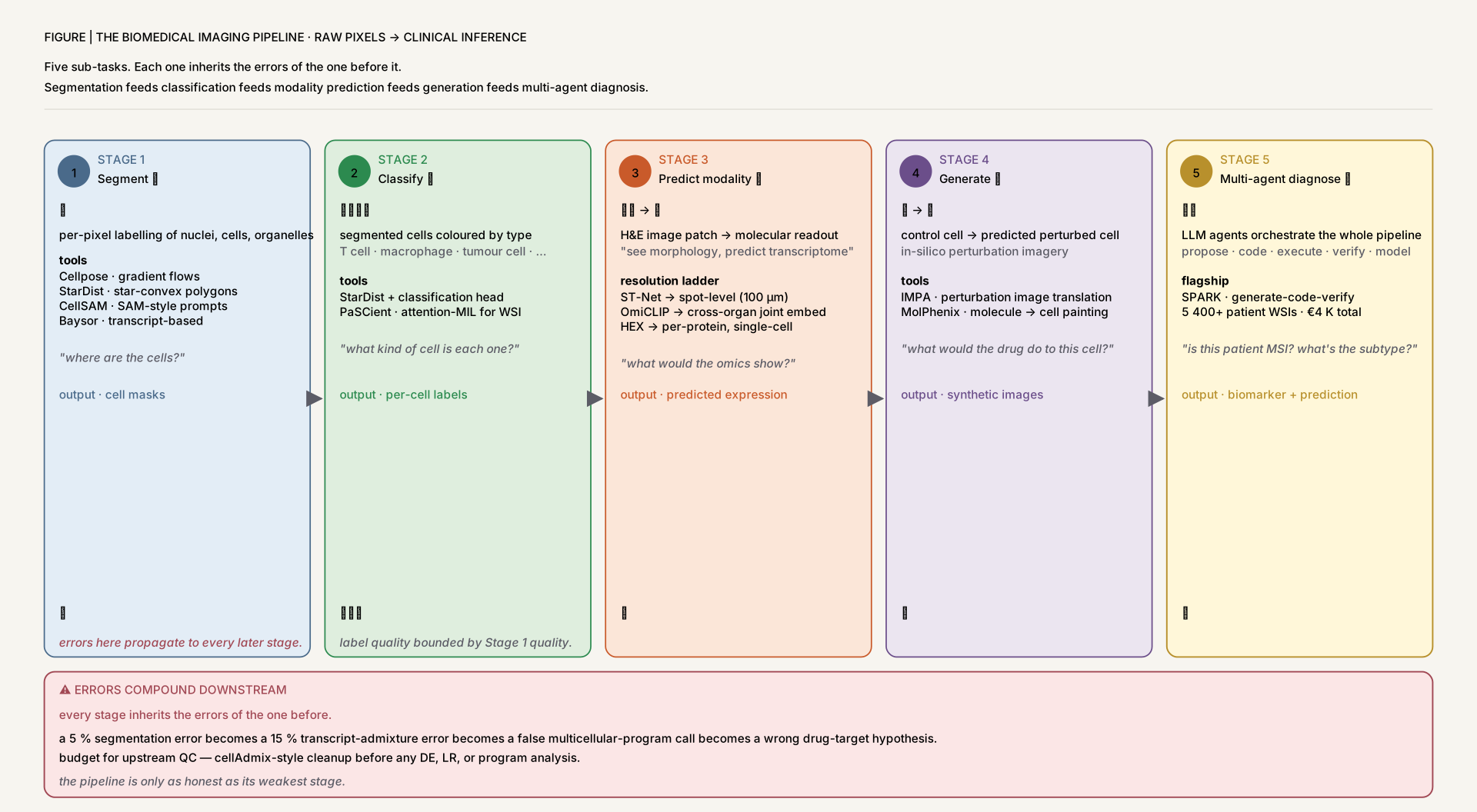
The five image-AI sub-tasks (segment / classify / predict modality / generate / multi-agent diagnose)
Segment. Per-pixel labelling. Cellpose (gradient flows, AP0.5 = 0.91), StarDist (star-convex polygons, mPQ = 0.5013 on CoNIC), CellSAM (SAM + CellFinder, F1-error 0.40 zero-shot on LIVECell), Baysor (Bayesian + MRF over transcripts, 2× more cells than DAPI-based), ESPRESSO (organelle-level with hyperspectral phasor unmixing). The substrate every other task builds on.
Classify. Single-cell or whole-slide labelling. StarDist with classification head (6 cell types, 1st place CoNIC 2022), Classpose (8% PQ improvement over Semantic CP-SAM across 6 datasets), PaSCient (135 disease states from 24.3M cells × 5,000 patients, weighted F1 = 0.70).
Generate. Synthesise perturbed cells or modality-translated images. IMPA (StarGAN-style perturbation prediction, FID +17% over StarGANv2), MolPhenix (CLIP-style retrieval of molecule given image, top-1% recall 77.3% vs 5.1% for CLOOME). See perturbation-modeling.html.
Multi-agent diagnose. LLM agents that orchestrate analytical pipelines over images. SPARK (1,115 verified parameters from H&E across 5 cancer types and 5,400+ patients, MSI AUROC 0.933). See ai-agents.html.
Figure 1The biomedical imaging pipeline — raw pixels to clinical inference. Five sub-tasks. Each one inherits the errors of the one before it. Segmentation feeds classification feeds modality prediction feeds generation feeds multi-agent diagnosis. The most important consequence: if you don't audit stage 1, every downstream metric is contaminated. This is why cellAdmix exists.
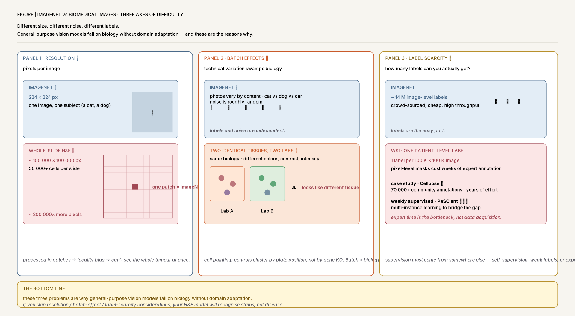
Why biological images are harder than ImageNet (resolution, batch effects, low labels)
Resolution mismatch. ImageNet is 224×224 of a single object. A whole-slide H&E image is 100,000×100,000 pixels with 50,000+ cells; a Xenium FOV may contain ~700K transcripts. Patch-based pipelines are mandatory, which means downstream models inherit the patch's locality bias (ST-Net's 100µm spots average over tens of cells; HEX uses 224×224 tiles for 40 protein channels).
Batch effects dominate. Cell painting plates, microscope channels, scanner colour profiles, and staining protocols all leak signal that swamps biology if not controlled. Spatial transcriptomics across slides has the same problem (Novae explicitly bakes optimal-transport batch correction into pretraining). CellPaint-POSH's CP-DINO needed defocus + coarse-dropout augmentation to handle this; cross-link to sc_batch_correction_integration.html.
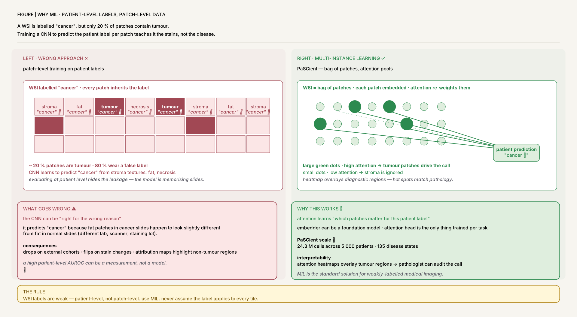
Labels are weak. Pixel-level masks are expensive (Cellpose's 70K+ annotations were a community effort over years). WSI labels are patient-level, not patch-level — that's why PaSCient uses MIL. Spatial-transcriptomics ground truth has only ~3,400 counts per spot in the original ST data; ST-Net trains on 23 patients total. The signal-to-noise is closer to medical imaging than to web data.
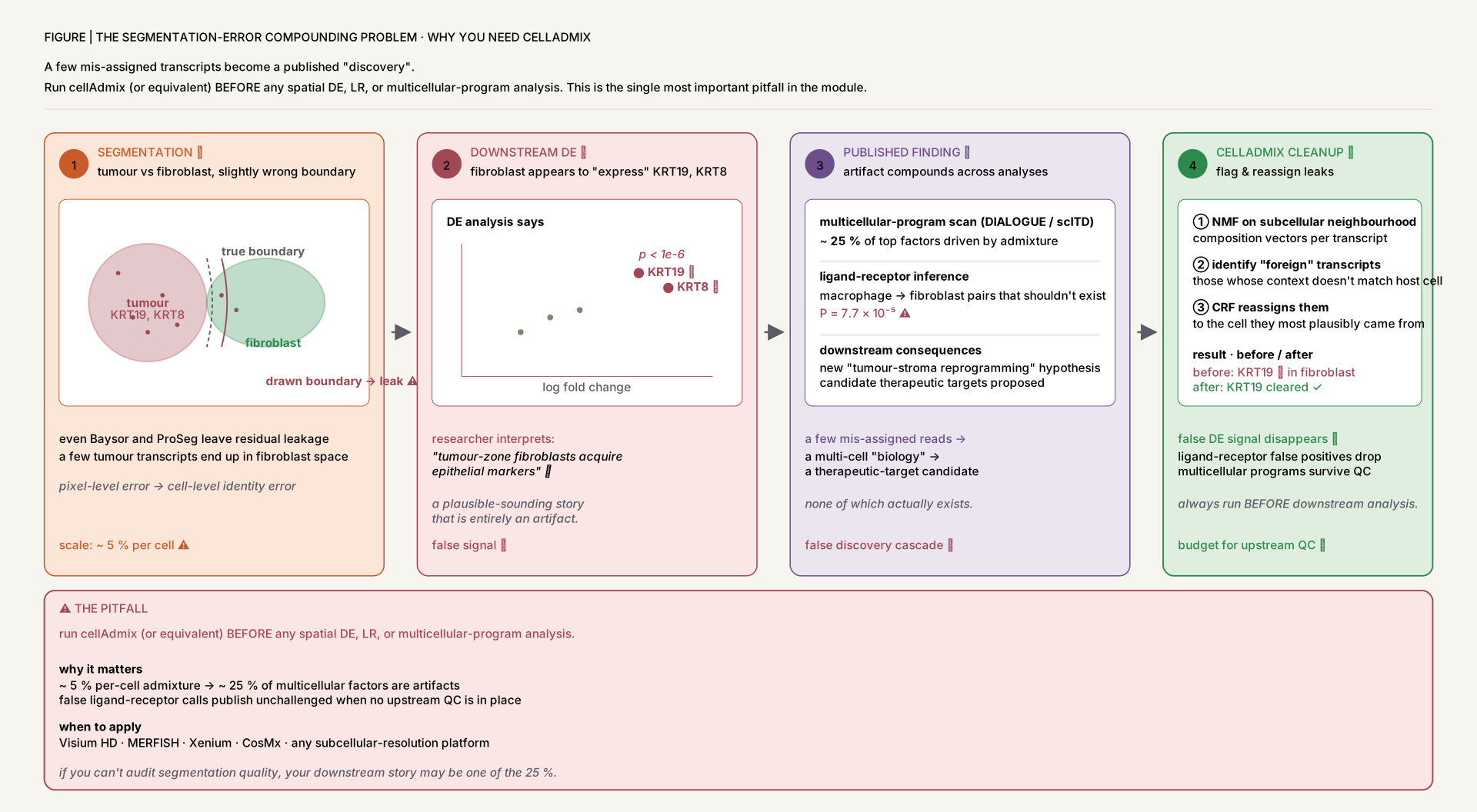
Segmentation errors compound. cellAdmix (Nat Genet 2026) showed every state-of-the-art segmenter (Baysor, BIDCell, ProSeg, 10x Multimodal) leaves cells contaminated with foreign transcripts, and that this contamination drives ~25% of published DIALOGUE/scITD factors and inflated ligand-receptor calls. A 5% segmentation error becomes a fundamentally wrong biological conclusion downstream.
Figure 2ImageNet vs biomedical images — three axes of difficulty. Different size, different noise, different labels. General-purpose vision models fail on biology without domain adaptation — and these are the reasons why. Every method in this module is doing something to handle at least one of these three axes; the strongest methods (Cellpose, CellSAM, Novae) handle all three.
Evolution Timeline
2020 — The two foundations: spatial profiling + H&E→ST
NanoString DSP (Nat Biotech) launches photocleavable-oligo digital spatial profiling on FFPE — 44 proteins or 1,412+ genes per ROI. ST-Net (Nat Biomed Eng) is the first paper to predict spatially resolved gene expression directly from H&E images via DenseNet-121, RMSE 0.31 on 250 genes, generalising zero-shot to 10x Visium and TCGA.
2021 — Generalist cell segmentation
Cellpose (Nat Methods) reframes segmentation as a vector-flow problem learned from simulated heat diffusion. AP0.5 = 0.91 across cytoplasm, brightfield, membrane, and even non-microscopy images — the first model that doesn't need retraining per dataset.
CosMx SMI (Nat Biotech) achieves 980 RNAs + 108 proteins at subcellular resolution in FFPE, with 0.0092 false calls per cell. Baysor (Nat Biotech) finds 2× more cells than DAPI-based segmentation by jointly modelling transcript composition and morphology. Squidpy (Nat Methods) ships the technology-agnostic spatial-omics framework. StarDist gets a classification head and wins CoNIC 2022 (mPQ 0.5013). Hist2ST adds Convmixer + Transformer + GNN to the H&E→ST recipe.
10x's serial-section study (Nat Commun) combines scFFPE-seq + Visium CytAssist + Xenium on the same breast cancer tissue, discovering rare "boundary cells" and a triple-positive region only detectable when 86% of Xenium cells are matched to scFFPE cell types.
2024 — Spatial clustering at scale + cell-painting goes contrastive + patient-level WSI
BANKSY (Nat Genet) unifies cell typing and tissue-domain segmentation by augmenting expression with neighborhood features and Gabor filters; processes 2M cells, 10–1000× faster than competitors. MolPhenix (NeurIPS) introduces contrastive PhenoMolecular Retrieval (top-1% recall 77.3%, 8.1× over CLOOME). PaSCient (bioRxiv) shows patient-level disease classification from 24.3M cells across 135 disease states.
2025 — Foundation models, generative perturbation, agentic platforms
CellSAM (Nat Methods) brings SAM + CellFinder to human-level segmentation across tissue, yeast, bacteria. OmiCLIP (Nat Methods) is the first CLIP-style visual-omics foundation model on 2.2M H&E–ST pairs. GHIST (Nat Methods) predicts single-cell SGE from H&E. ESPRESSO (Nat Methods) is the first organelle-level spatiotemporal omics (3,328 features/cell, 24h live). CellNEST (Nat Methods) detects multi-hop relay LR networks with GAT+DGI. Novae (Nat Methods) pretrains a graph-FM on 29M cells across 18 tissues. CellPaint-POSH (Nat Commun) marries 5-channel Cell Painting with pooled CRISPR + ISS + DINO-ViT (1,640-gene druggable genome). MedMPT (Nat Biomed Eng) builds a chest-CT vision-language model. IMPA (Nat Commun) generates perturbed cell images via style transfer. Classpose extends Cellpose-SAM to H&E phenotyping. SpatialEx anchors multi-omics integration on H&E + UNI foundation features.
HEX (Nat Med) predicts 40 protein biomarkers from H&E at Pearson r 0.73–0.79, beating cGAN by 46%; +22% prognosis, +24–39% immunotherapy response prediction in NSCLC. cellAdmix (Nat Genet) quantifies and corrects segmentation-error admixture, showing ~25% of published spatial DIALOGUE/scITD factors are admixture artifacts. DBiTplus (Nat Methods) integrates spatial transcriptomics with CODEX/CellScape protein imaging on the same tissue via RNase H cDNA retrieval. SPARK (Nat Med) is the first multi-agent LLM "pathology brain" — 1,115 verified concepts, 5 cancer types, 5,400+ patients, MSI AUROC 0.933, reconstructs tumor-evolution chains from static H&E.
Side-by-Side: Supervised Regression vs Contrastive Pretraining for H&E → Gene Expression
ST-Net and OmiCLIP both map the same H&E tile to a molecular readout, but they diverge on every key design axis: label representation (continuous per-gene counts vs ranked gene-sentence tokens), training objective (MSE regression vs contrastive image–text alignment), and scale (23 patients vs 1,007 samples across 32 organs).
Same input — a 224×224 H&E tile from a Visium slide — becomes very different model inputs and outputs:
multi-scale global · contrastive self-supervised · panel-agnostic · gene-sentence tokens
The split traces back to one root decision — what is the label? ST-Net treats the molecular readout as 250 continuous regression targets and pays the price of a fixed gene panel and spot-averaged resolution. OmiCLIP reframes the same data as a language-vision alignment problem: the top-50 expressed gene names become a "sentence," and contrastive learning forces the image embedding and gene-sentence embedding to agree — unlocking panel-agnostic transfer across 32 organs, retrieval, annotation, and decomposition without retraining.
Method Families
Grouped by the AI task and substrate. Within each family, papers are ordered chronologically. Several papers span families (e.g., CellSAM is both segmentation and foundation model); they are placed in the better-fitting family and cross-referenced.
1. Cell & Organelle Segmentation (7)
Per-pixel labelling. The substrate every downstream task depends on. From U-Net + gradient flows (Cellpose) to star-convex polygons (StarDist) to Bayesian transcript-aware models (Baysor) to foundation-model promptable segmentation (CellSAM, Classpose) to organelle-resolution hyperspectral imaging (ESPRESSO) to post-segmentation cleanup (cellAdmix).
Cellpose: a generalist algorithm for cellular segmentation
2021Nat MethodsU-Net + gradient flow
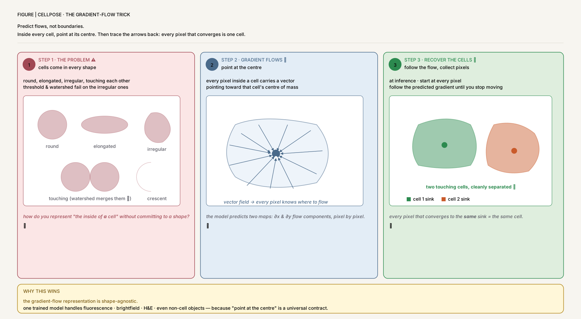
Cellpose reframes instance segmentation as a "follow-the-flow" problem: a modified U-Net predicts simulated-diffusion gradient fields plus inside/outside probability, then test-time pixels are clustered by tracking gradients to common fixed points. Trained on 608 mixed fluorescent, brightfield, membrane and non-microscopy images. Style-vector conditioning enables one model to generalise across modalities without retraining; 2D model extends to 3D by averaging xy/xz/yz gradients.
AP0.5 = 0.91 specialised, 0.77 generalised — vs StarDist 0.76/0.61 and Mask R-CNN 0.80/0.61
485/521 ground-truth ROIs correctly matched with only 18 false positives on specialised data
3D segmentation of 190µm3 mouse cortex: 172 cells predicted vs 183 ground truth, 17 FPs at IoU=0.5
Adding non-biological images (rocks, jellyfish, fruits) to training improves generalisation — the model learns object-ness, not cell-ness
Figure 3Cellpose — the gradient-flow trick. Predict flows, not boundaries. Inside every cell, point at its centre. Then trace the arrows back: every pixel that converges is one cell. The trick is that gradient fields are dense (every interior pixel has a target vector) where boundaries are sparse (only thin contours have positive labels), so the supervision signal is much richer. This is what lets Cellpose generalise across modalities a boundary-supervised method couldn't.
Cell segmentation in imaging-based spatial transcriptomics (Baysor)
2022Nat BiotechBayesian + MRF
Baysor is a Bayesian mixture model that segments cells in MERFISH, smFISH, ISS, STARmap directly from transcript positions, with optional auxiliary membrane stain. Each cell is modelled as 2D/3D Gaussian over positions plus a Categorical over gene identity, with a Potts MRF prior for spatial coherence. The Neighborhood Composition Vector (NCV) trick enables segmentation-free visualization before committing to boundaries.
Up to 2× more cells than DAPI-based segmentation (osmFISH); 42% more endothelial cells in hypothalamus MERFISH (long morphology → nuclei often outside imaging plane)
Higher fraction of molecules assigned to cells than Watershed or pciSeq across 5 protocols
51 min for 3.7M molecules (MERFISH), 40.4 GB memory for 1,020-gene STARmap
Recovers vascular and astrocytic cells missed by nuclei-only methods (only 10% captured in original osmFISH segmentation)
Nuclei Instance Segmentation and Classification in Histopathology with StarDist
2022ISBIStar-convex polygons
StarDist is extended for histopathology by adding a semantic segmentation head to the existing star-convex polygon predictor: a U-Net backbone predicts per-pixel object probability, 64 radial distances per pixel, and 6 class probabilities. Per-instance class is the majority vote of pixel-level predictions. Wins CoNIC 2022 first place for joint nuclei segmentation and 6-class colon-cell classification.
1st place CoNIC 2022 final test: mPQ 0.5013, PQ 0.6607 across 6 cell types (neutrophil, epithelial, lymphocyte, plasma, eosinophil, connective)
Simple oversampling improves mPQ from 0.39 (no balancing) to 0.59 — beats focal loss (0.45) and class weights (0.51)
H&E-specific staining augmentation boosts external test mPQ from 0.36 to 0.43
Shape refinement via aggregated suppressed polygons improves segmentation quality beyond standard NMS
ESPRESSO: spatiotemporal omics based on organelle phenotyping
2025Nat MethodsHyperspectral + CNN
ESPRESSO is the first spatiotemporally resolved omics technique: 4-color live-cell hyperspectral confocal imaging (lysosome, mitochondria, lipid droplets, DNA) with phasor unmixing, CARE-denoised acquisition, Cellpose segmentation, and 3,328 morphological + functional features per cell. Tracks single-cell phenotype transitions for 24+ hours at 30-min resolution. Connects organelle landscape to cell state without genetic manipulation, applicable to 2D cultures, 3D spheroids, and across cell types.
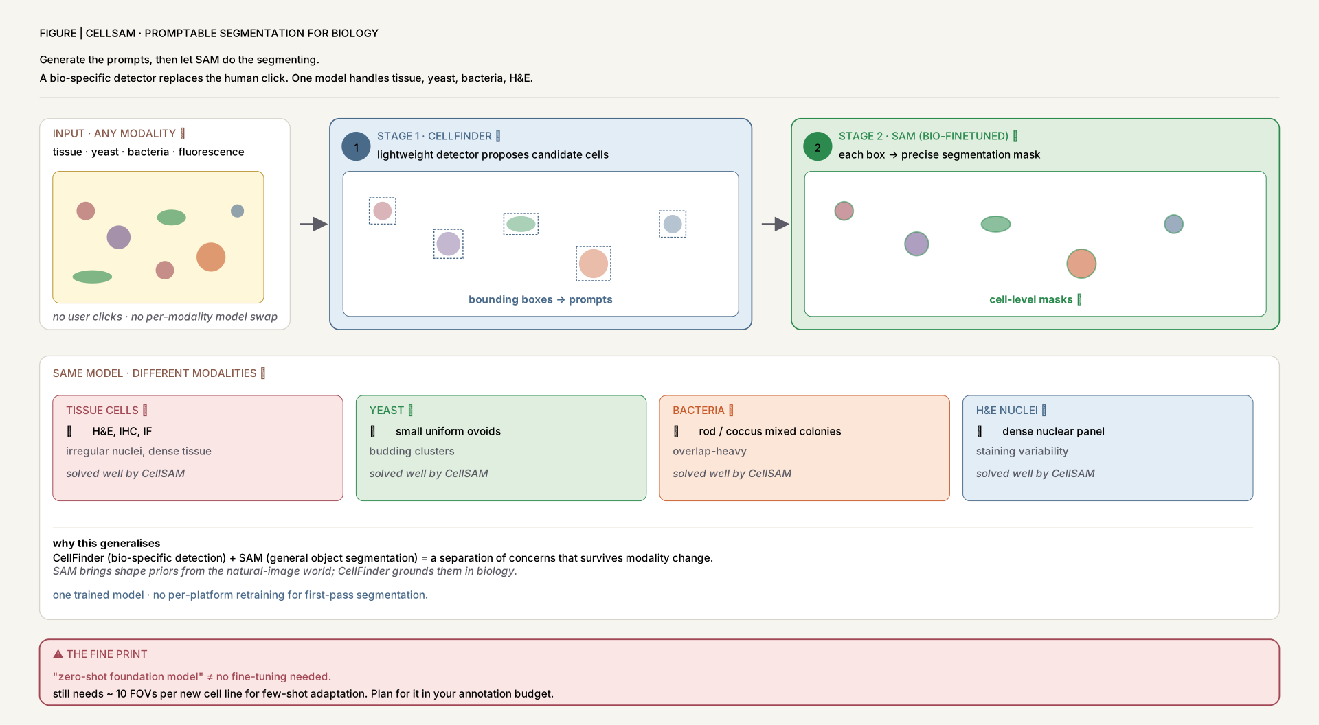
CellSAM extends Segment Anything Model (SAM) with CellFinder — an Anchor-DETR transformer object detector with 3,500 queries and NMS-free design — that auto-generates bounding-box prompts for SAM's mask decoder. Two-stage training: first CellFinder + ViT-B backbone on detection, then freeze ViT and fine-tune SAM neck. Trained on ~2M cell annotations across 10 datasets (tissue 975K, cell culture, H&E, bacteria, yeast, nuclear) including TissueNet, DeepBacs, BriFiSeg, Cellpose, Omnipose, YeastNet, YeaZ, DSB, H&E collections, Phase400.
Human-level accuracy: no significant difference between CellSAM/human and human/human (P = 0.18 tissue, 0.49 cell culture, 0.11 yeast, 0.90 bacteria)
Zero-shot LIVECell F1-error 0.40 vs Cellpose 0.60
First generalist that doesn't degrade when trained on more diverse data (Cellpose does)
Few-shot learning: performance improves with as few as 10 FOVs (~102–103 cells) per new cell line; integrates with Polaris for MERFISH/seqFISH
Figure 4CellSAM — promptable segmentation for biology. Generate the prompts, then let SAM do the segmenting. A bio-specific detector replaces the human click. One model handles tissue, yeast, bacteria, H&E. The trick that makes SAM useful for biology: SAM was trained to respond to prompts, not to generate them. CellFinder fills the gap with a domain-specific detector trained on cells specifically.
Classpose: foundation-model-driven WSI-scale cell phenotyping in H&E
2025bioRxivCellpose-SAM + multi-task
Classpose adds semantic cell-type classification to Cellpose-SAM via a "bag of tricks" approach: full-network fine-tuning, class-weighted sampling, hybrid losses (BCE + MSE for segmentation, multi-class CE + Focal Tversky for classification), learnable-sigma uncertainty-based loss weighting, extended H&E/HED augmentations, and sparse-annotation support. Tested on 6 datasets (CoNIC, ConSep, GlySAC, MoNuSAC, NuCLS, PUMA) for joint instance segmentation + cell-type classification at whole-slide scale.
Panoptic Quality +0.08 vs Semantic CP-SAM, +0.14 vs StarDist, +0.16 vs CellViT++ (P<0.0001) across 6 benchmarks
Full-network fine-tuning improves PQ from 0.134 (class head only) to 0.515
bf16 inference: 45% speedup with no performance loss
Ships CLI tool + QuPath extension; lymphocytes/inflammatory cells transfer best across datasets (consistent H&E morphology)
Impact and correction of segmentation errors in spatial transcriptomics (cellAdmix)
2026Nat GenetNMF + CRF cleanup
cellAdmix is the first post-segmentation cleanup analogous to scRNA-seq doublet filtering for imaging-based spatial transcriptomics. Builds molecule-level subcellular Neighborhood Composition Vectors (sNCVs), factorises them with weighted NMF, then a Conditional Random Field over the molecular k-NN graph assigns each transcript to a factor. A novel reference-free cell-bridging test identifies which factors are "foreign" to the host cell and strips those transcripts. Quantifies segmentation-error damage across 6 datasets and 4 segmenters (Baysor, BIDCell, ProSeg, 10x Xenium Multimodal).
~25% of top DIALOGUE/scITD multicellular factors are admixture-driven artifacts
NSCLC fibroblast DE: 11/36 top upregulated genes were malignant markers (KRT19, KRT8) — lose significance after cleaning
Giotto-predicted macrophage→fibroblast LR pairs enriched for fibroblast marker ligands (COL6A3, BGN, DCN; hypergeometric P = 7.7×10⁻⁵) — large share of published spatial cell-cell communication calls likely artifactual
P_admix significantly reduced (P<10−3) for all 12 NSCLC cell types; 98% of cells lose <10% of native transcripts
Figure 5The segmentation-error compounding problem — why you need cellAdmix. A few mis-assigned transcripts become a published "discovery". Run cellAdmix (or equivalent) BEFORE any spatial DE, LR, or multicellular-program analysis. This is the single most important pitfall in the module — every method downstream of segmentation can amplify a small boundary error into a wrong biological conclusion.
2. H&E → Spatial Expression Prediction (6)
Learn the H&E↔molecular bridge. From the seminal CNN ST-Net (250 genes from 100µm spots) through transformer + GNN hybrids (Hist2ST) to single-cell-resolution multi-task UNet 3+ (GHIST), CLIP-style 2.2M-pair foundation models (OmiCLIP), hypergraph H&E-anchored multi-omics (SpatialEx), and virtual proteomics for clinical biomarkers (HEX).
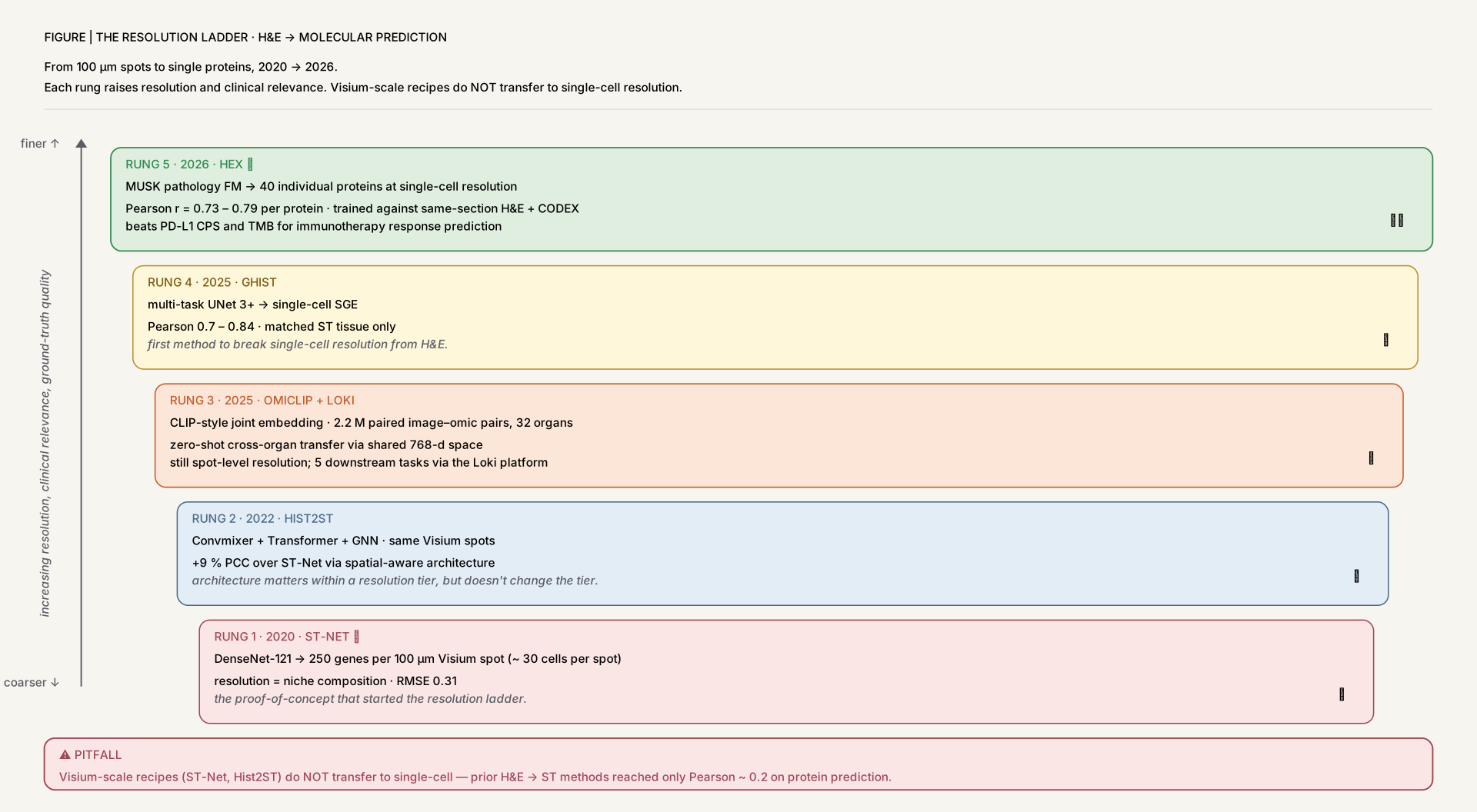
Figure 6The resolution ladder — H&E → molecular prediction, 2020 → 2026. From 100µm spots to single proteins. Each rung raises resolution and clinical relevance. Visium-scale recipes do NOT transfer to single-cell resolution — moving up the ladder is not a hyperparameter change but a pipeline redesign.
Integrating spatial gene expression and breast tumour morphology via deep learning (ST-Net)
2020Nat Biomed EngDenseNet-121 multi-task
The original H&E→spatial expression paper. ST-Net is a DenseNet-121 with ImageNet pre-training that takes 224×224-pixel (~150×150µm2) H&E patches centred on Spatial Transcriptomics spots and predicts log-normalised expression of 250 target genes via a shared 1,024-dim representation + per-gene fully-connected head. Trained on 23 breast cancer patients (3 sections each) with leave-one-patient-out CV. Generalises zero-shot to 10x Visium and 1,550 TCGA bulk samples.
RMSE 0.31, AUROC 0.73 average across 234 genes on independent 10x Visium
102/250 genes predicted with positive correlation in >=20/23 patients (FDR 0.05); top genes are cancer biomarkers (GNAS, FASN, DDX5, XBP1, ACTG1)
207/234 genes positive correlation on 10x; 177/249 on TCGA bulk
Tumour vs immune co-localization reduced (P<0.001) — consistent with 75% of breast cancer patients having low TILs
Hist2ST: Spatial transcriptomics prediction from histology via Transformer and GNN
2022Brief BioinformConvmixer + Transformer + GNN
Hist2ST is a three-module architecture: Convmixer (depthwise + pointwise convolutions, kernel=7, stride=7) for 2D vision features within each H&E patch, an 8-layer 16-head Transformer for global spot-to-spot dependencies (with 2D coordinate encoding), and a 4-layer GraphSAGE GNN with LSTM aggregation for local 4-neighbor relationships. Output is a ZINB layer predicting zero-inflated counts. Self-distillation handles limited ST training data.
+9% mean PCC vs HisToGene on HER2+ breast cancer; +11% on cSCC
+7.6–19% PCC across Alzheimer's, mouse brain, olfactory bulb datasets
Spatial-region detection ARI +7% vs HisToGene, +5% vs observed gene expression — predictions add information beyond ground truth
Works across 10x Visium, ST-seq, Space-TREX, Stereo-seq platforms; identifies disease-relevant FN1, GNAS, SCD, MYL12B
OmiCLIP: A visual-omics foundation model bridging histopathology and spatial transcriptomics
2025Nat MethodsCLIP-style 2.2M pairs
OmiCLIP is the first CLIP-style foundation model trained on 2,185,571 H&E–transcriptomics paired tiles from 113 public 10x Visium studies across 32 organs. Treats spatial transcriptomics as "sentences" of top-50-expressed genes per spot, aligned with 224×224 H&E tiles via a CoCa-based dual encoder (ViT image encoder + causal-masking text encoder, 768-d shared space, 20 epochs, batch 64). Ships the Loki platform with 5 modules (Align, Annotate, Decompose, Retrieve, PredEx) for downstream use.
GHIST: Spatial gene expression at single-cell resolution from histology
2025Nat MethodsUNet 3+ multi-task
GHIST is the first method to predict single-cell spatial gene expression from H&E (not spot-level). UNet 3+ backbone (5 feature scales, full-scale skip connections) jointly learns nuclei segmentation/classification, cell type, neighborhood composition, and gene expression via cross-attention (8 heads). Trained on subcellular spatial transcriptomics (Xenium-style) to capture interdependencies between morphology, cell type, niche, and expression.
Cell-type accuracy 0.75 (BreastCancer1) and 0.66 (BreastCancer2) across 8 cell types
SpatialEx: High-parameter spatial multi-omics through histology-anchored integration
2025Nat MethodsUNI + hypergraph
SpatialEx and SpatialEx+ use H&E as a universal anchor for spatial diagonal integration: Cellpose segments cells, the UNI pathology foundation model embeds each cell's H&E patch, a hypergraph encoder (k=7 nearest neighbors per hyperedge, two-stage node↔hyperedge message passing) captures group-level interactions, and contrastive learning with a corrupted hypergraph captures global context. SpatialEx+ adds an Omics Cycle Module to integrate different single-omics measurements from serial sections without requiring simultaneous coprofiling.
CMD 0.206 vs DeepPT 0.302 vs CNN_Reg 0.271 (lower better) for H&E→omics prediction
+28–66% NMI for spatial domain identification vs DeepPT
Scales to >1M cells; works at spot and single-cell resolution without modification
Demonstrates panel diagonal integration (Xenium 313 genes split 150 + 163 across sections) and omics diagonal (metabolomics + transcriptomics on Parkinson's mouse brain)
HEX: AI-enabled virtual spatial proteomics from histopathology for lung cancer
2026Nat MedMUSK FM + regression
HEX generates virtual 40-protein CODEX from standard H&E using the MUSK pathology foundation model (pretrained on 50M images + 1B text tokens, multi-scale 10x/20x/40x) followed by a 3-layer regression head (embedding→256→128→40) with Feature Distribution Smoothing and Adaptive Loss Function. Same-section H&E + CODEX co-staining gives pixel-level ground truth; 224×224 tiles at 40x. Validated on NLST training (414), TCGA, PLCO, Stanford-TMA, TA-TMA, and Stanford-IO immunotherapy cohort (2,150 patients total).
The platforms that produce multiplexed tissue data and the software that processes them. DSP (44 proteins or 1,412 genes from FFPE ROIs), CosMx SMI (980 RNAs + 108 proteins at subcellular resolution), DBiTplus (sequencing + multiplexed imaging on same section), and the integration ecosystem: Squidpy (technology-agnostic analysis), BANKSY (spatial clustering at scale), CellNEST (GAT-based multi-hop relay LR networks), and the Xenium-Visium-scFFPE breast cancer reference study.
Multiplex digital spatial profiling of proteins and RNA in fixed tissue (DSP)
2020Nat BiotechPhotocleavable DSP
NanoString GeoMx Digital Spatial Profiling uses photocleavable oligonucleotide tags + DMD (digital micromirror device) UV projection at 365 or 385 nm to release indexing oligos from user-selected ROIs on standard FFPE tissues. Read out via nCounter (direct fluorescent barcode counting) or NGS with i5×i7 indexing. ROIs can be any shape from single cells to ~5,000 cells, even non-contiguous. Single-cell sensitivity for protein, ~600-transcript sensitivity for RNA.
44 proteins or 96 genes (nCounter); 1,412 genes / 4,998 probes (NGS); LOD 1.3–3.7 cells for high-expressors
Works directly on FFPE archival samples (no fresh-frozen required); ~1 µm2 per micromirror
Cross-platform R2 0.93–0.98 vs RNAscope; R2>0.8 nCounter vs NGS
~384 ROIs per 48h workflow; demonstrated immune contexture mapping in CRC and IBD
Squidpy: a scalable framework for spatial omics analysis
2022Nat MethodsPython analysis FW
Squidpy is the Python framework that unifies spatial omics analysis across Visium, seqFISH, MERFISH, SlideseqV2, IMC, 4i, MIBI-TOF. Two main data structures: a spatial neighborhood graph from coordinates (grid/generic, KNN/radius/Delaunay) and an ImageContainer with on-disk/in-memory switching for very large microscopy images. Numba JIT compilation gives ~10× speedup over Giotto. Integrates with Scanpy/AnnData ecosystem and napari for interactive visualization.
~10× faster neighborhood enrichment than Giotto; scales to ~270K subcellular observations
Spatial statistics: Moran's I, Ripley's L/F/G, co-occurrence, neighborhood enrichment z-scores
Re-implements CellPhoneDB ligand-receptor with Omnipath; image features include Haralick texture, summary, histogram, deep-learning extraction
Backends for StarDist and Cellpose segmentation; works across spot-based, single-cell, and subcellular (4i) resolution data
High-resolution mapping of the TME using integrated single-cell, spatial and in situ analysis (Xenium-Visium-scFFPE)
2023Nat CommunTri-platform integration
10x Genomics' reference study integrating three FFPE technologies on serial breast cancer sections: Chromium scFFPE-seq (18,536 genes, median 1,480 genes/cell), Visium CytAssist (whole-transcriptome spots), and Xenium In Situ (313-gene panel, subcellular resolution, 167,885 cells, median 166 transcripts/cell). All three share the same probe set, enabling "spot interpolation" — using Xenium to derive whole-transcriptome info for spatially-identified rare cell populations.
86% of Xenium cells unambiguously matched to scFFPE-seq cell types; r2=0.99 serial-section correlation
Xenium 8.4× higher median gene sensitivity than Visium in shared capture area
BANKSY: unifies cell typing and tissue domain segmentation for spatial omics
2024Nat GenetSpatial clustering
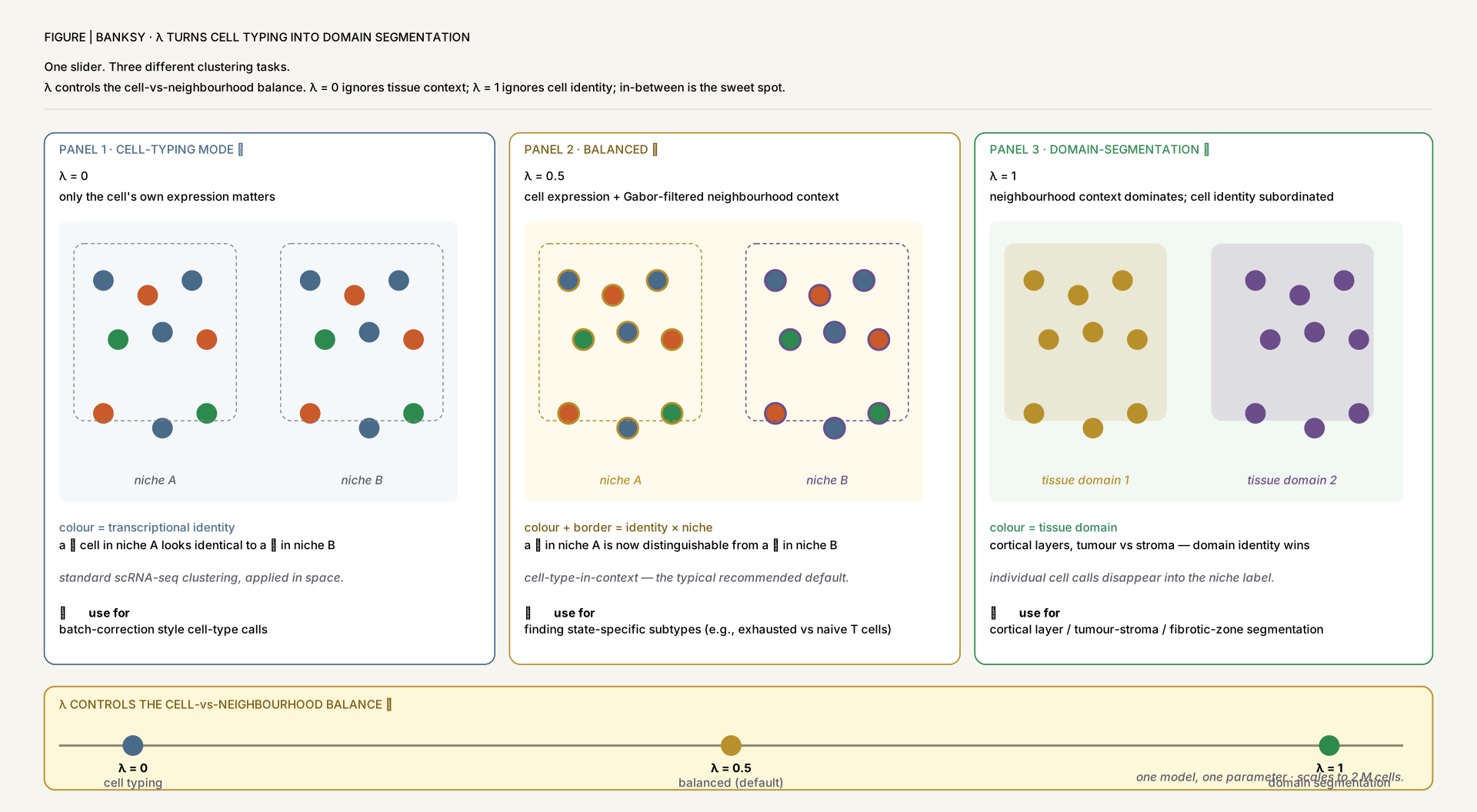
BANKSY augments each cell's gene expression vector with two neighborhood features: mean weighted neighborhood expression and an azimuthal Gabor filter (AGF) capturing expression gradients. The augmented matrix B = [√(1−λ)·C; √(λ/μ)·M; √(λ/2μ)·G] is reduced via PCA (20 PCs) and clustered with Leiden. A single λ parameter switches between cell typing (λ≈0.2) and tissue-domain segmentation (λ≈0.8). Cross-link to cell-annotation_type-identification.html.
10–1000× faster than existing spatial clustering; 2–60× more scalable (processes 2M cells; competitors fail at 250–500K)
DLPFC ARI 0.518 across 12 samples (tied best with GraphST, STAGATE); STARmap ARI 0.720 (highest)
Discovers niche-dependent oligodendrocyte subtypes (white vs gray matter, Mbp/Lpar1 vs Mlc1/Gad1) and cycling epithelial cells in CRC missed by non-spatial methods
Works across MERFISH/MERSCOPE (RNA imaging), Slide-seq/Visium (RNA seq), CODEX (protein imaging); median ARI IQR 0.015 across 65 parameter combinations
Figure 7BANKSY — λ turns cell typing into domain segmentation. One slider. Three different clustering tasks. λ controls the cell-vs-neighbourhood balance. λ = 0 ignores tissue context; λ = 1 ignores cell identity; in-between is the sweet spot. Sweeping λ on the same dataset is a cheap way to ask "is this a cell-type signal, a niche signal, or both?"
CellNEST: cell-cell relay networks using attention on spatial transcriptomics
2025Nat MethodsGAT + Deep Graph Infomax
CellNEST is the first deep learning method to detect single-cell-resolution multi-hop relay LR networks (Cell A → ligand → Cell B receptor → ligand → Cell C) in spatial transcriptomics. Multi-edge graph where edges encode [distance, L-R coexpression, L-R pair ID]; GAT encoder with Tanh activation; Deep Graph Infomax contrastive learning (Jensen-Shannon divergence) overcomes lack of CCC ground truth; 5-run ensemble with rank-product aggregation. Cross-link to sc_cell_cell_communication_methods.html.
Balanced accuracy 0.8–1.0 across 21 synthetic benchmarks vs 0.2–0.6 for 6 competitors (NICHES, COMMOT, CellChat, Giotto, CytoSignal, NicheCompass, TWCOM)
CCL19–CCR7 T-cell homing in human lymph nodes: Fisher's P = 9.16×10−224; detects relay to CCL21–CXCR4
Only method to systematically validate relay networks against STRING + NicheNet + DoRothEA databases
Works on Visium (55µm), Visium HD (2µm), MERFISH (single-cell), 3D MERFISH; PDAC subtype-specific signals (PLXNB2–MET in classical, ANXA1–EGFR in basal-like, P=4.02×10⁻²⁵)
DBiTplus: imaging-based + sequencing-based spatial omics on the same tissue section
2026Nat MethodsRNase H cDNA retrieval
DBiTplus runs DBiT-seq spatial barcoding (50 channels × 50 channels, 25–50 µm resolution), then uses thermostable RNase H at 55°C to enzymatically release cDNA — preserving tissue morphology for subsequent CODEX or CellScape multiplexed protein imaging on the same section. Computational integration via MaxFuse + RCTD-like imaging-guided spot splitting into pure cell-type sub-spots. Compatible with OCT-frozen and FFPE archival samples.
20,973–27,884 genes detected per experiment; ~1,200 genes and 3,300 UMIs per spot (E11 mouse embryo)
R=0.99 vs standard DBiT-seq; RNase H preserves 14/25 CODEX markers vs poor staining with NaOH/DMSO
TACCO deconvolution: >0.6 Pearson correlation in 50% of spots vs ground truth
Applied to mouse embryo (26-marker CODEX), human lymph node (35-plex), and lymphoma progression (MZL, Richter's transformation) revealing IL6ST/CLU/NFKBIA, ROR2/SMOC2 programs
Pretrained encoders trained on massive paired image-omics or image-only datasets that transfer zero-shot to new tissues, panels, and cancer types. CellSAM (Family 1), OmiCLIP (Family 2) are also foundation models; this section features the general-purpose histopathology encoders (UNI, CONCH, GigaPath, PLIP) that most 2024–2026 downstream work — including SpatialEx and HEX elsewhere in this module — builds on, plus Novae, the graph-based spatial-transcriptomics FM. Cross-link to sc-foundation-models.html and pretraining.html.
UNI: a general-purpose self-supervised model for pathology
2024Nat MedDINOv2 ViT-L
UNI is a ViT-L/16 encoder pretrained with DINOv2 self-supervision on Mass-100K, a de-identified corpus of >100,000 diagnostic H&E whole-slide images (>100M tissue patches) spanning 20 major tissue types from Massachusetts General Brigham. It is the reference general-purpose tile encoder cited by SpatialEx elsewhere in this module ("UNI + hypergraph") and by many pathology FM downstream pipelines that need frozen patch embeddings rather than a vision-language joint space.
Evaluated zero-shot/few-shot and via linear probing on 34 clinical tasks: tissue classification, cancer subtyping, and slide-level retrieval
Outperforms prior supervised (ImageNet) and self-supervised (CTransPath, REMEDIS) pathology encoders on the majority of benchmarked tasks, including several rare cancer subtypes
Ships as a frozen feature extractor — most downstream work (MIL classifiers, hypergraph encoders like SpatialEx) treats UNI embeddings as fixed input rather than fine-tuning end-to-end
CONCH: a visual-language foundation model for computational pathology
2024Nat MedCoCa vision-language
CONCH is a CoCa-style vision-language foundation model pretrained on >1.17M histopathology image–caption pairs sourced from educational material (textbook figures, PubMed Open Access articles) rather than clinical WSIs directly, avoiding the patient-data-sharing constraints that limit purely image-only corpora. It jointly learns an image encoder and a text encoder in a shared embedding space, enabling zero-shot classification and text-to-image/image-to-text retrieval — the capability Novae elsewhere in this module optionally uses for H&E fusion ("Optional H&E fusion via CONCH embeddings").
State-of-the-art zero-shot and few-shot performance across 14 downstream tasks spanning tissue classification, tumor detection, and cross-modal retrieval
Zero-shot classification without any task-specific fine-tuning, by prompting with class-name text rather than training a linear probe
Vision-language joint space makes CONCH embeddings usable both as image features and for text-guided retrieval, unlike image-only encoders like UNI
Prov-GigaPath: a whole-slide foundation model for digital pathology from real-world data
2024NatureViT + LongNet, 1.1B params
GigaPath is the first foundation model to pretrain on true whole-slide images rather than independently sampled tiles: a tile-level ViT encoder (DINOv2) first embeds 256×256 patches from 171,189 WSIs (>1.3B patches) across 30,000+ patients and 31 tissue types from the Providence health network, then a slide-level LongNet transformer with dilated attention aggregates all of a slide's tile embeddings — up to tens of thousands of tiles — into a single whole-slide representation, capturing long-range spatial dependencies that tile-only encoders (UNI, CONCH) discard.
Outperforms prior slide-level MIL/foundation-model baselines across 25+ downstream tasks including cancer subtyping, mutation prediction, and treatment response
First large-scale demonstration that whole-slide (not just tile-level) self-supervised pretraining transfers to real-world clinical cohorts, not just curated benchmark sets
LongNet's dilated attention makes slide-level self-attention computationally tractable at the tens-of-thousands-of-tiles scale a full WSI produces
PLIP: a visual-language foundation model for pathology image analysis using medical Twitter
2023Nat MedCLIP fine-tune
PLIP (Pathology Language and Image Pre-training) fine-tunes CLIP on OpenPath, >200,000 pathology image–text pairs mined from medical-education Twitter/X accounts and public pathology forums — the first demonstration that social-media-scale (not institutional-WSI-scale) paired data could train a usable pathology vision-language model. PLIP is the direct architectural predecessor to CONCH, and remains a widely used baseline for zero-shot pathology image retrieval and classification in the downstream literature.
Zero-shot classification competitive with, and in some tasks exceeding, models trained on much larger proprietary WSI corpora, at a fraction of the data-curation cost
Cross-modal retrieval: given a pathology image, retrieve semantically matching text descriptions and vice versa, without task-specific training
Demonstrated that social-media pathology discourse (case discussions, teaching images) is a viable, low-cost alternative data source to institutional WSI archives — a data-sourcing strategy later scaled up by CONCH's curated educational corpus
Novae: a graph-based foundation model for spatial transcriptomics
2025Nat MethodsGraph FM + SwAV
Novae is a self-supervised graph attention network for spatial transcriptomics, pretrained on ~29M cells across 78 slides, 18 tissues, 3 technologies (Xenium, MERSCOPE, CosMx). Delaunay graph (edges >80µm truncated), 2–3-edge local subgraphs, panel-invariant gene embeddings (L2-normalized weighted sum initialized from scGPT) so the same model works across different gene panels. SwAV-style swapped-prediction loss with K trainable prototypes (elementary spatial domains) and optimal-transport batch correction baked in — no external Harmony needed. Optional H&E fusion via CONCH embeddings.
Highest FIDE (domain continuity) and JSD (cross-slide homogeneity) on breast, colon, synthetic datasets; ARI 0.8+ on synthetic vs <0.6 for STAGATE/GraphST/SpaceFlow/SEDR
Processes 6.4M cells in ~10 seconds for batch correction + domain assignment (vs days for Harmony + Leiden)
Zero-shot mode beats trained competitors on real datasets; pretrained model on Hugging Face Hub
Reveals shared domains across lymph node + tonsil, cancer-related domains shared between lung and breast tumors; H&E integration identifies bronchus-specific domain (D2032) missed by single modalities
Image-based phenotypic profiling at compound or genetic-perturbation scale. CellPaint-POSH (DINO-ViT on 5-channel + ISS-based CRISPR readout, 1,640-gene druggable genome), MolPhenix (CLIP-style molecule↔image retrieval), IMPA (generative perturbation imagery via StarGAN). Cross-link to perturbation-modeling.html and contrastive-learning.html.
How Molecules Impact Cells: Contrastive PhenoMolecular Retrieval (MolPhenix)
2024NeurIPSCLIP-style retrieval
MolPhenix introduces zero-shot Contrastive PhenoMolecular Retrieval: given a Cell Painting phenomic image, retrieve the correct molecular structure. Embeds both modalities in a joint latent space using Phenom1 (masked autoencoder for phenomics) + MolGPS (GNN for molecules), with a novel Soft-weighted Sigmoid Locked (S2L) loss combining SigLIP label-noise robustness and CWCL inter-sample similarity. Explicit (log/sigmoid/one-hot) and implicit concentration encoding handle dosage-dependent effects.
Top-1% retrieval recall 77.33% on active molecules vs CLOOME 5.06% — 8.1× improvement
Unseen dataset (RXRX3) recall: MolPhenix 58.6% vs CLOOME 2.07%
S2L loss outperforms CLIP, InfoLOOB, CWCL, SigLIP across all cumulative and held-out tasks
Zero-shot perturbation matching infers gene knockout↔drug relationships; KNN on embeddings beats standalone fingerprints on TDC and Polaris property prediction
IMPA: Predicting cell morphological responses to perturbations via generative modeling
2025Nat CommunStarGAN-style cGAN
IMPA is a conditional GAN with content encoder, style encoder, condition encoder, and multi-task discriminator (separate classification head per condition). AdaIN style conditioning with adversarial + style consistency + cycle consistency + style diversification losses. Unified perturbation embedding handles chemical (Morgan Fingerprints, 1024d), CRISPR (Gene2Vec + HyenaDNA, 328d), and ORF overexpression (456d) within one framework, plus learnable batch embeddings for batch correction.
FID +17% improvement over StarGANv2; +45% average improvement on batch correction metrics
Chemical-space interpolation enables unseen-compound prediction via Tanimoto similarity; perturbation space clusters drugs by functional similarity despite chemical distance
Single model performs both perturbation prediction and technical-variation correction
CellPaint-POSH: pooled Cell Painting CRISPR + self-supervised DL
2025Nat CommunDINO-ViT + ISS
CellPaint-POSH combines pooled CRISPR knockout (A549 cells, CROPseq-like vector), a 5-stain Cell Painting panel (Hoechst, ConA, WGA, Phalloidin, Mitoprobe-Cy5 RNA-FISH) that is compatible with 4-color in situ sequencing for sgRNA barcode decoding, and CP-DINO (DINO-v1 ViT-Small, 21.86M params, 384-dim CLS, patch=8) trained self-supervised on 1.59M single-cell tiles. Replaces stress-inducing MitoTracker with Mitoprobe (mt-rRNA FISH) for ISS compatibility. Druggable-genome scale demonstrated at 1,640 genes.
Druggable genome (1,640 genes): 113 genes with KO-vs-intergenic AUC>0.6 (CP-DINO 1640) vs 95 (CP-DINO 300); ~5.6M cells imaged
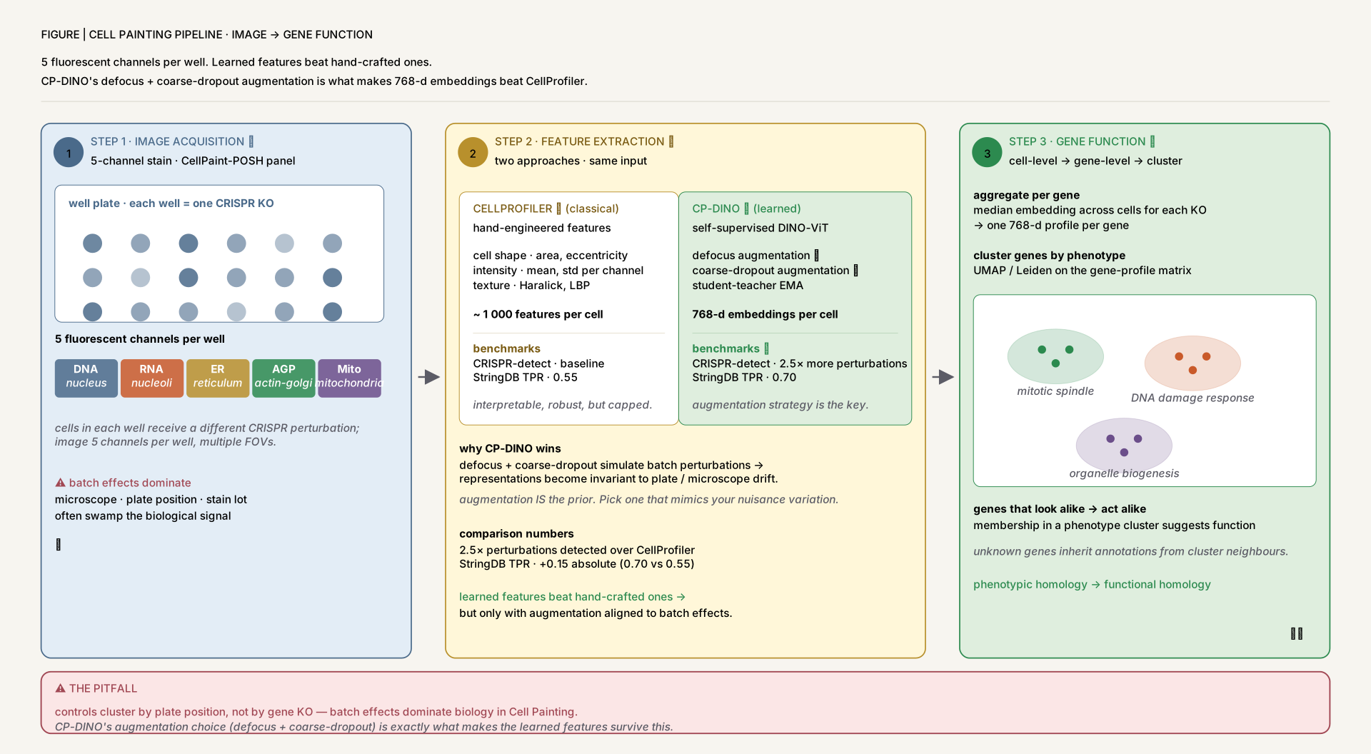
Figure 8Cell Painting pipeline — image to gene function. 5 fluorescent channels per well. Learned features beat hand-crafted ones. CP-DINO's defocus + coarse-dropout augmentation is what makes 768-d embeddings beat CellProfiler. The augmentation choice is doing real biological work — it teaches the encoder to be invariant to optical artifacts (defocus) and partial-cell occlusion (coarse-dropout), both of which plague Cell Painting plates.
6. Histopathology & Whole-Slide Imaging (1)
WSI-scale analysis. Patient-level disease state from millions of cells across 5,000+ patients via Multi-Instance Learning. HEX (Family 2) and Classpose (Family 1) are also WSI methods; SPARK (Family 7) operates at WSI scale via agents. Cross-link to transfer-learning.html and embedding-strategies.html.
PaSCient: Multi-cellular representations for patient-level disease states
2024bioRxivMulti-Instance Learning
PaSCient is a DeepSet-inspired patient-level model with a cell embedder (Rd_g → Rd_h), attention aggregator (w_i = softmax(a_θ(Z_i)), e_i = w_iTZ_i), and disease classifier MLP. Trained end-to-end on 24.3M cells from CELLxGENE across 135 unique disease states, 5,000+ patients, 189 tissues, 413 studies, with disease + tissue oversampling for class balance. Multi-level splits ensure no study leakage between train/val/test. Integrated gradients enable cell, gene, and cell-type-specific interpretability.
Weighted F1 = 0.70 for 135-class disease classification (vs 0.60 for best baseline)
COVID-19 severity: 88% accuracy vs 79% for pseudo-bulk; beats CellPLM, SCimilarity, ScRAT
Non-linear attention +16.6% over mean pooling; transformer overparameterized for this task
Gene-prioritization significantly overlaps with ToppCell DEGs (P<2.1×10⁻²²); generalizes out-of-study on 4 independent COVID severity cohorts
Figure 9Why MIL — patient-level labels, patch-level data. A WSI is labelled "cancer", but only 20% of patches contain tumour. Training a CNN to predict the patient label per patch teaches it the stains, not the disease. MIL with attention pooling is the load-bearing architecture for any patient-level prediction from WSIs — PaSCient is the cell-level version; classic Camelyon17-style WSI work is the patch-level version. The general lesson: align label granularity with prediction granularity, or pay an interpretability tax forever.
7. Multimodal & Agentic Diagnosis (2)
Image + text + workflow. From paired chest-CT-report vision-language pretraining at clinical scale (MedMPT) to multi-agent LLM systems that autonomously generate, code, and verify analytical hypotheses across cancer cohorts (SPARK). The clinical-deployment edge of biomedical imaging. Cross-link to ai-agents.html, attention-mechanisms.html, retrieval-augmented-generation-bio.html, and reasoning-llms-biology.html.
MedMPT: vision-language pretrained transformer for respiratory disease
2025Nat Biomed EngChest-CT VLM
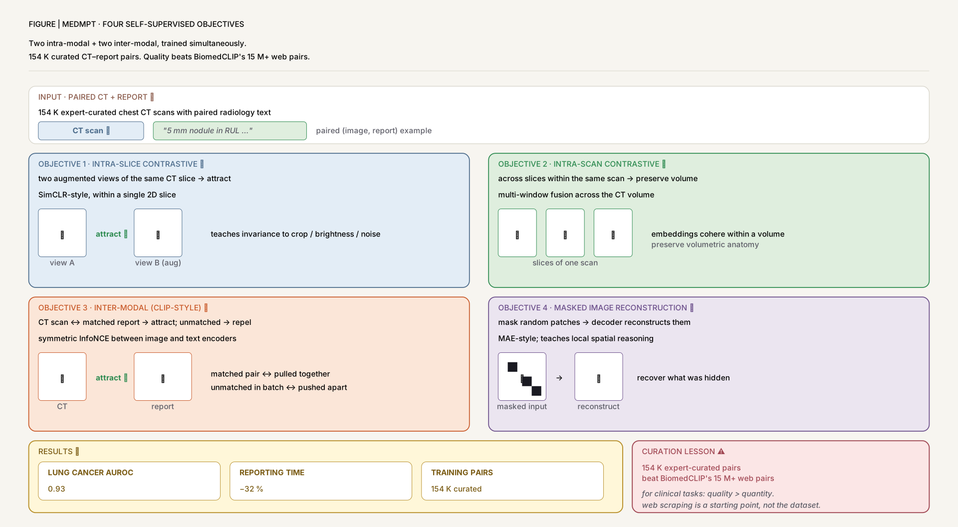
MedMPT pretrains on 154,274 chest-CT–radiology-report pairs via four complementary self-supervised objectives: intramodal contrastive (slice + scan, momentum encoder m=0.996), intermodal contrastive (CT ↔ report), masked image reconstruction (20% mask), and cross-modal generation. Vision encoder is a ViT-based slice encoder + self-attention slice-fusion that treats the CT as a unified 3D volume rather than independent 2D slices. Downstream: disease diagnosis, zero-shot report generation, and prescription recommendation augmented with a medication co-occurrence graph attention network.
Figure 10MedMPT — four self-supervised objectives, trained simultaneously. Two intra-modal + two inter-modal. 154 K curated CT–report pairs. Quality beats BiomedCLIP's 15 M+ web pairs. This is the same MedMPT lesson that appears in the pretraining module's "curated vs massive" pitfall — when labels are clinical and noise is structured, curated data wins.
SPARK: agentic framework for autonomous discovery in cancer pathology
2026Nat MedMulti-agent LLM
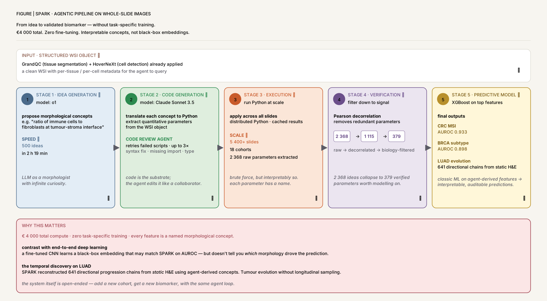
SPARK is a multi-agent LLM "pathology brain" built on crewAI. Specialized agents (OpenAI o1 for ideation, o3-mini for review/dedup, Claude Sonnet 3.5 for coding) generate biologically motivated H&E hypotheses, refine them into executable specs, write Python that operates on a preprocessed WSI object (GrandQC tissue detection + UNet++/EfficientNet organ-specific segmentation + HoverNeXt single-cell classification into 7–8 cell types), and verify across cohorts. Outputs concept-level interpretable parameters — not embeddings — that map back to specific cells and spatial relationships. Zero task-specific model retraining required.
1,115 verified parameters from 475 ideas across 5 cancer types and 5,400+ patients in 18 cohorts; full development cost ~€4,000
CRC MSI status AUROC 0.933; BRCA subtype 0.898; ER status 0.863; HNSC HPV/p16 status 0.828 — matches or exceeds SOTA
Discovers cross-tumor "active tumor front" signature (neutrophils + eosinophils + fibroblasts at tumor–stroma interface) shared across LUAD/LUSC/COAD
Reconstructs tumor evolution from static H&E: 40,721 directional pairs in LUAD → 641 aggressiveness chains; first cohort-scale static-image temporal-dynamics inference
Figure 11SPARK — agentic pipeline on whole-slide images. From idea to validated biomarker — without task-specific training. €4 000 total. Zero fine-tuning. Interpretable concepts, not black-box embeddings. The deliverable shape (concept-level parameters that map back to specific cells) is what makes SPARK's output usable clinically; an end-to-end embedding model would have produced the same AUROCs but no mechanistic story.
Selection at a Glance
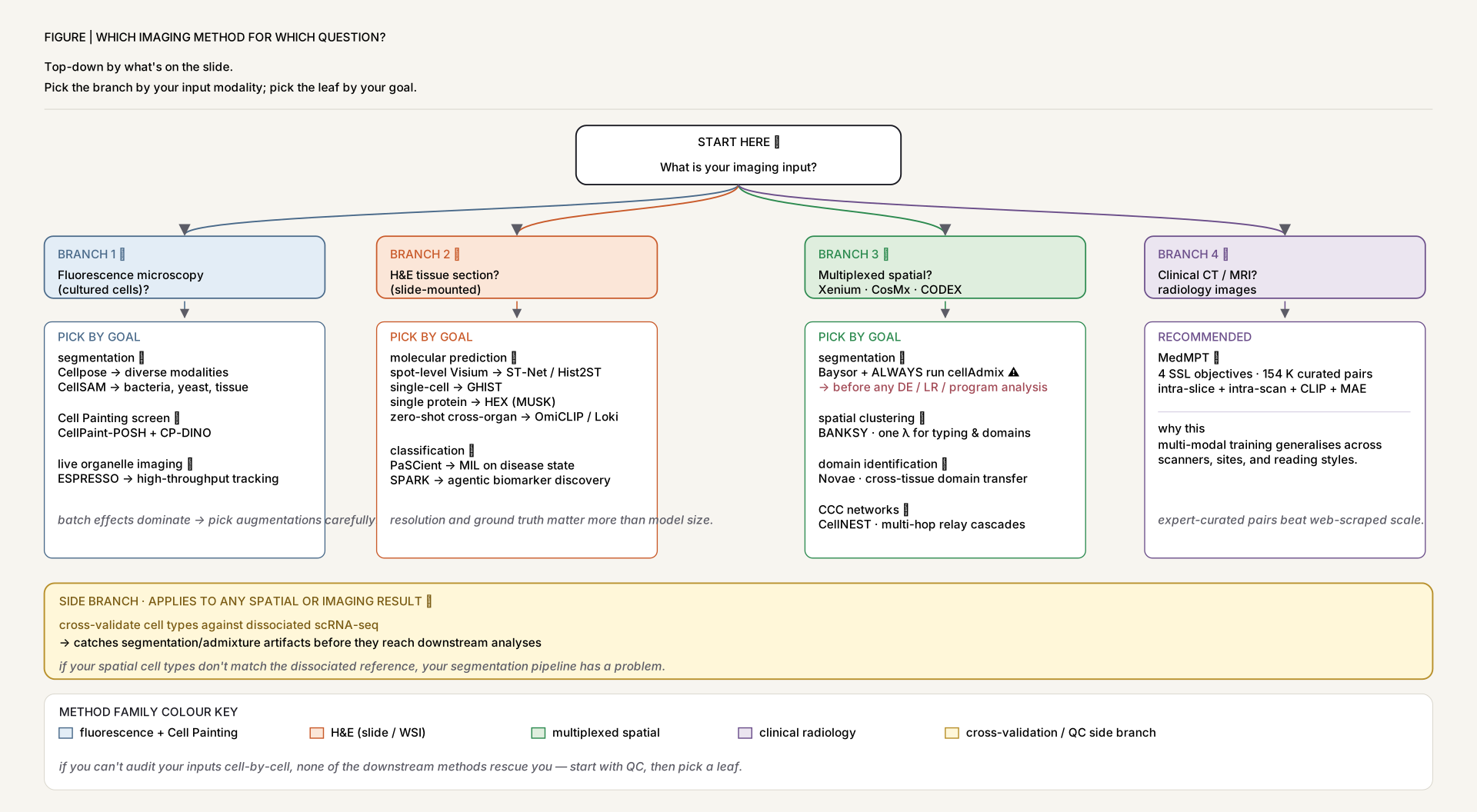
Quick reference: which imaging recipe to reach for given your task, modality, and label budget.
Figure 12Which imaging method for which question? Top-down by what's on the slide. Pick the branch by your input modality; pick the leaf by your goal. The most common mistake in this literature is reaching for the trendiest method (CellSAM, OmiCLIP, SPARK) before checking whether the leaf-level method for your specific task already exists and works.
Start here. The clearest demonstration of how a single deep-learning model can generalise across diverse microscopy. The gradient-flow trick is intuitive; the dataset construction philosophy (include non-cell objects for object-ness) shapes every later foundation model.
2. ST-Net (2020, Nat Biomed Eng)
The original H&E→spatial expression paper. Read it before any later H&E→ST work to understand what 250 genes / 100µm / RMSE 0.31 actually looks like, and why DenseNet-121 + multi-task learning was the right starting point.
3. Squidpy (2022, Nat Methods)
The framework that makes everything in this module composable. Understand the spatial neighborhood graph + ImageContainer abstraction; almost every later paper assumes one of these.
Read these as a pair. Baysor is the "right" way to segment imaging-based ST; cellAdmix is the reality check: even the best segmenter leaves cells contaminated enough to drive ~25% of downstream multicellular-factor findings. This is the most important pitfall in the whole module.
5. CellSAM + OmiCLIP (2025, Nat Methods)
The two foundation-model shifts. CellSAM brings SAM-style promptable segmentation to bio; OmiCLIP brings CLIP-style joint embedding to H&E + ST at 2.2M scale. Read together to see how vision-foundation-model patterns map onto biology.
6. HEX (2026, Nat Med) and SPARK (2026, Nat Med)
Where the field is going clinically. HEX shows that virtual molecular readouts from routine H&E can beat established biomarkers (PD-L1, TMB) for immunotherapy response. SPARK shows that LLM agents can do interpretable cohort-scale biomarker discovery autonomously. Both are this year; both will reshape pathology.
Practical Implementation Guide
If your goal is single-cell segmentation in microscopy
Start with Cellpose (use the GUI, set the diameter, done). If the model fails, try fine-tuning with Cellpose 2.0 human-in-the-loop, or escalate to CellSAM for very diverse modalities (tissue/yeast/bacteria/H&E in one). For dense histopathology nuclei with cell-type classification, use StarDist with classification head or Classpose. For dense imaging-based spatial transcriptomics, use Baysor (transcripts alone) or Baysor + membrane stain — and always run cellAdmix afterwards to remove molecular admixture artifacts.
If your goal is WSI classification or biomarker prediction
For patient-level disease state from scRNA-seq cell bags, use PaSCient's attention-based MIL. For direct H&E→molecular prediction, the choice depends on resolution: ST-Net / Hist2ST for spot-level (100µm), GHIST for single-cell, HEX for protein readouts. For zero-shot use across organs, OmiCLIP's Loki platform. For agentic discovery across multi-cohort H&E, SPARK — but budget the LLM API costs (~€4,000 for full development) and remember the outputs are interpretable concepts, not embeddings.
If your goal is multiplexed tissue analysis
Pick a platform: DSP for archival FFPE with whole-transcriptome ROIs, CosMx SMI or Xenium for subcellular RNA + protein, DBiTplus if you need spatial transcriptomics + multiplexed protein on the same section. For analysis, use Squidpy as the spine, BANKSY for cell typing + domain segmentation at scale (millions of cells), Novae for zero-shot domain identification across slides/panels, and CellNEST for ligand-receptor relay networks. Always validate against the Xenium-Visium-scFFPE breast cancer benchmark study before trusting cell-type assignments. Cross-link to spatial-transcriptomics.html.
If your goal is high-content / cell-painting screening
For pure morphology readout, use CellPaint-POSH's 5-channel panel with CP-DINO embeddings — the self-supervised DINO-ViT beats hand-crafted CellProfiler features (StringDB TPR 0.70 vs 0.55 on held-out 124-gene POC) and detects 2.5× more perturbations than CellProfiler on external PERISCOPE data. For predicting perturbed cell images (in-silico screening), use IMPA's StarGAN-style generation — chemical-space interpolation enables unseen-compound prediction. For phenotype-to-molecule retrieval, use MolPhenix's contrastive approach (top-1% recall 77.3%). For organelle-resolved temporal profiling without genetic engineering, ESPRESSO's 4-color hyperspectral + 3,328 features per cell.
Common Pitfalls
Cell painting batch effects dominate biological signal. Microscope, plate, well position, and stain lot effects routinely swamp gene-knockout signals in Cell Painting. CellPaint-POSH needed defocus + coarse-dropout + dropout augmentation in DINO training to make CP-DINO work; IMPA needed an explicit batch-correction module. Always check that PCA on your control wells separates by batch before you trust any gene-level signal.
WSI labels are weak — patient-level, not patch-level. A diagnosis label applies to the entire slide, but only some patches contain the diagnostic feature. Standard patch-level training will memorise noise. Use Multi-Instance Learning (PaSCient-style attention aggregation) or hierarchical foundation models; never train a patch-level classifier on patient-level labels and then evaluate at the patient level — you will hide the leakage.
H&E→spatial expression only works at low-resolution Visium scale. ST-Net and Hist2ST work because 100µm spots contain tens of cells — the model is really predicting niche composition. At true single-cell Xenium resolution, only GHIST and HEX (which leverages a pathology foundation model and the same-section CODEX ground truth) work, and HEX explicitly notes that prior H&E→ST methods reached Pearson ~0.2 on protein prediction while HEX reaches 0.73–0.79. Don't expect Visium-scale recipes to transfer.
Pathology FMs trained on TCGA fail on rare cancers. Foundation models inherit pretraining-corpus bias. MUSK, CONCH, UNI are all heavy on common cancers (BRCA, LUAD, CRC, prostate). On rare entities (NUT carcinoma, mesothelioma subtypes), zero-shot performance drops sharply. Always validate on a held-out cohort containing your target tumor type before deploying clinically; this is one reason SPARK explicitly verifies parameters per cancer type.
Segmentation errors compound through downstream pipelines. The cellAdmix paper is the single most important caveat in this module: even state-of-the-art segmenters (Baysor, BIDCell, ProSeg, 10x Multimodal) leave cells contaminated. Tumor-zone fibroblast DE picks up malignant markers (KRT19, KRT8) that are just neighbor admixture. ~25% of top DIALOGUE/scITD multicellular factors are admixture artifacts. Run cellAdmix or an equivalent post-segmentation cleanup before any spatial DE, ligand-receptor, or multicellular-program analysis.
"Foundation model" does not mean "no fine-tuning needed". CellSAM still needs few-shot adaptation (~10 FOVs) per new cell line. OmiCLIP needs domain-specific fine-tuning for performance ceilings on rare organs. HEX needed fine-tuning on colorectal cancer to improve prediction for 57 markers. Plan for a small labelled validation set and a fine-tune budget even when using "zero-shot" foundation models.
Curated clinical pairs beat web scale. MedMPT showed 154K expert-curated chest-CT/report pairs beat BiomedCLIP's 15M+ web pairs on clinical tasks. The same pattern recurs: high-quality paired data (HEX's same-section H&E + CODEX, OmiCLIP's curated 2.2M Visium pairs) beat naive scaling. Budget for curation, not scraping, when your target task is clinical.
Don't trust a single platform's cell-type assignment. The 2023 Xenium-Visium-scFFPE study found ~14% of Xenium cells could not be unambiguously matched to scFFPE-seq cell types — and ~1% were "boundary cells" coexpressing tumor and myoepithelial markers that mattered biologically. Always cross-validate spatial cell-type calls against dissociated scRNA-seq (or vice versa) on the same patient.
Hands-On Practice
This walkthrough takes you from a raw biomedical image (fluorescence microscopy or H&E) to a segmented, classified result using the core libraries in the field. All snippets are self-contained and can be adapted to DICOM clinical images, NIfTI MRI/CT volumes, or whole-slide SVS files by swapping the loader shown in the Data Structures section.
Environment & packages
Install into a fresh Python 3.10 environment. MONAI covers clinical volumetric imaging; cellpose handles fluorescence/H&E cell segmentation; tiatoolbox is the recommended WSI pipeline; SimpleITK and nibabel cover DICOM and NIfTI I/O respectively.
Hardware. Cellpose and StarDist run comfortably on CPU for small images (<1024×1024). For MONAI 3-D models or WSI tile inference, a GPU with ≥8 GB VRAM is strongly recommended; use torch.cuda.is_available() to verify before starting.
Data structures & formats
NumPy arrays (H, W, C) or (C, H, W) — the universal in-memory format; channel order matters (scikit-image uses HWC, PyTorch uses CHW).
DICOM (.dcm) — clinical CT/MRI scans stored slice-by-slice; load with pydicom.dcmread() or SimpleITK.ReadImage(); always read PixelSpacing and SliceThickness metadata — physical voxel size drives all morphology measurements.
NIfTI (.nii / .nii.gz) — standard for MRI/CT volumes after DICOM conversion; load with nibabel.load(); affine matrix encodes voxel-to-world-space mapping — never ignore it.
OME-TIFF / SVS (whole-slide images) — multi-resolution pyramidal tiles up to ~100,000×100,000 px; access with tiatoolbox.wsicore.WSIReader or openslide.OpenSlide; always specify the magnification level (e.g., 20×) rather than a pixel level index, as level 0 differs between scanners.
PNG/TIFF fluorescence stacks — 2-D or 3-D multichannel microscopy; load with skimage.io.imread() (TIFF) or tifffile.imread() for multi-page/hyperstack files.
Segmentation masks — integer-labelled arrays where 0 = background and each positive integer is a unique cell/instance ID; distinct from semantic masks (class IDs only, no instance distinction).
Minimal code walkthrough
Load a fluorescence image, normalise it, run Cellpose instance segmentation, then measure per-cell mean intensity — a typical starting point for any cell-biology screen.
import numpy as np
from skimage import io, exposure
from skimage.measure import regionprops_table
from cellpose import models
import pandas as pd

# 1. Load — shape (H, W) grayscale or (H, W, C) multichannel
img = io.imread("cells_DAPI.tif")          # uint16 or uint8 fluorescence TIFF

# 2. Normalise to [0, 1] using 1st–99th percentile clip (avoid outlier saturation)
p1, p99 = np.percentile(img, (1, 99))
img_norm = exposure.rescale_intensity(img, in_range=(p1, p99))

# 3. Cellpose segmentation — "nuclei" model for DAPI; set diameter to measured nucleus size in px
model = models.Cellpose(gpu=True, model_type="nuclei")
masks, flows, styles, diams = model.eval(
    img_norm,
    diameter=30,        # estimate from scale bar or CellProfiler "MeasureObjectSizeShape"
    channels=[0, 0],    # grayscale: [chan_of_interest, chan_for_nucleus_or_0]
    flow_threshold=0.4,
    cellprob_threshold=0.0,
)

# 4. Measure per-cell features using regionprops
props = regionprops_table(
    masks,
    intensity_image=img_norm,
    properties=["label", "area", "mean_intensity", "eccentricity", "bbox"],
)
df = pd.DataFrame(props)
print(df.head())

# 5. Quick QC — remove cells touching the image border and very small debris
border_labels = set(np.unique(masks[0, :])) | set(np.unique(masks[-1, :])) \
              | set(np.unique(masks[:, 0])) | set(np.unique(masks[:, -1]))
df = df[~df["label"].isin(border_labels) & (df["area"] > 100)]
print(f"Cells passing QC: {len(df)}")
Common pitfalls & tips
Always read pixel spacing / voxel size metadata. DICOM PixelSpacing and NIfTI affine matrices encode physical scale. Skipping them means your area, diameter, and volume measurements are in pixel units — meaningless across scanners or magnifications. Use SimpleITK.GetSpacing() or nibabel.load().header.get_zooms() to extract it before any morphology measurement.
Set Cellpose diameter correctly or let it estimate. Leaving diameter=None triggers auto-estimation but adds ~20 s per image; too-small values over-segment, too-large values merge nuclei. Measure 10–20 representative cells with ImageJ/FIJI first, then fix the diameter for reproducibility across a batch.
Tile WSIs at the right magnification and with overlap. In tiatoolbox, always request tiles at a named magnification (e.g., power=20) rather than a pyramid level. Use at least 64 px overlap on each edge and stitch predictions with weighted blending or Gaussian feathering — hard-edge tiling produces grid artefacts in both segmentation masks and feature maps.
Normalise H&E stain before deep models. Macenko or Vahadane stain normalisation (available in tiatoolbox.tools.stainnorm) reduces scanner-to-scanner colour variation by ~40% on CoNIC-style benchmarks; without it, a model trained on one scanner fails on another. Apply normalisation before any patch extraction step.
Patient-level data leakage is the most common evaluation error. If a patient has 50 WSI tiles and you randomly split tiles into train/test, the model memorises patient appearance. Always split at the patient (or slide) level; use stratified splits to balance disease class across folds.
Class imbalance in histology is severe. In CoNIC, neutrophils are <2% of nuclei; in PaSCient, rare disease classes have <50 patients. Use class-weighted sampling, Focal loss, or Focal Tversky loss (as in Classpose) rather than standard cross-entropy, and always report per-class F1 rather than macro accuracy — a model predicting "lymphocyte" for every nucleus can look 70% accurate while being useless.