∫ Optimal Transport & Wasserstein Distance in Single-Cell Biology
Mathematical & Algorithmic Foundations for Cellular Distribution Analysis
A rigorous guide to optimal transport theory and Wasserstein metrics in computational biology.
From mathematical foundations (Monge, Kantorovich, entropic regularization) to modern applications
in trajectory inference, multi-omics integration, and distributional comparison. Covering landmark
methods (Waddington-OT, moscot, SCOT) and theoretical advances (2019-2025).
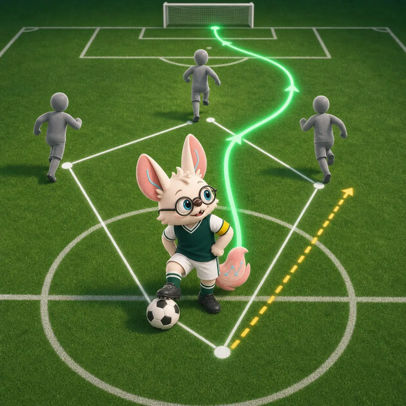
Football lens · optimal transport
球不是带过去的,是传过去的。
Move the whole team, not one player. A build-up from goalkeeper to striker is a transport problem: every pass has a price, and the cheapest plan is always a team effort. 把一堆细胞从 A 状态搬到 B 状态,最省的路径不是逐个点对点,而是一张全局的传球网络。
⚽ Build-Up Play: Optimal Transport in Six Moves
「最便宜的推进,是全队的传球网络。」
Optimal transport asks how to move an entire distribution for the least total cost. A football build-up asks the same: get the ball from your box to theirs, through eleven players, at the lowest risk per meter. Six moves from the training ground, re-read as the math in this module.
Move 1 · 阵型图 The formation sheet
Two distributions
Before kickoff the analyst pins two sheets: our shape, their shape. Eleven dots each — but the dots carry weight, and the weights sum to the whole squad.
Source and target. μ and ν are two formations of cell states: positions plus masses. OT starts from both full distributions, never a handful of star players.
Move 2 · 每脚传球都有代价 Every pass has a price
The cost matrix
A five-yard square pass is cheap; a sixty-yard diagonal over the press is expensive. The coach prices every lane before choosing one — distance, pressure, interception risk.
Ground cost c(x,y). The price of moving one unit of mass from x to y. Distances must be measured in a space where they mean something — PCA space, a latent embedding, or a graph metric.
Move 3 · 个人盘带不如全队推进 Dribbling is not a plan
Coupling
The highlight-reel dribble past five men loses the ball nine times out of ten. The cheap build-up is boringly global: every player where the plan needs him, every pass the simple one.
Coupling π(x,y). The optimal plan is a joint distribution — how much mass from each source cell lands on each target cell. Greedy nearest-neighbour choices do not add up to the cheapest plan (Monge relaxes to Kantorovich).
Move 4 · 安全球与冒险球 The safe pass and the risky one
Entropic regularization
Every manager trades risk for tempo: all safe passes and you never progress; all Hollywood balls and you keep losing it. A dial between them sets the team's passing temperament.
Sinkhorn's ε. Entropic regularization blurs the plan for computability — the larger ε, the safer and more diffuse the passing lanes. The Sinkhorn cost is not the raw Wasserstein distance; it is biased by the blur.
Move 5 · 换人之后 After the substitutions
Unbalanced OT
Two substitutions change the squad on the pitch — the formation you planned for no longer has the same headcount. The plan must allow players to arrive and leave.
Unbalanced OT. Cells divide and die, so the two distributions need not weigh the same. Relax exact mass conservation with KL penalties, letting the plan create and destroy mass.
Move 6 · 叠两张阵型图 Overlaying two sheets
Alignment (moscot)
Video night: overlay our shape from the first leg on their shape from the second — who matched whom, and which matchups won the tie?
Distribution alignment. moscot couples cell populations across timepoints and conditions; fused Gromov–Wasserstein when the feature spaces differ. This is the workhorse for trajectory and integration.
Build-up play in four moves. Every pass has a price (the cost matrix) · dribbling is not a plan (greedy carry vs global coupling) · safe ball, risky ball (entropic regularization) · overlay the two sheets (distribution alignment with moscot).
「最便宜的推进从来不是英雄盘带,是全队的传球网络。」 — the cheapest move is a coupling, not a carry.
🎯 Core Concepts
What is Optimal Transport?
Optimal transport theory provides a mathematical framework for comparing probability distributions
by computing the minimal "cost" of transforming one distribution into another. Originally formulated
by Gaspard Monge in 1781 and generalized by Leonid Kantorovich in 1942, the theory asks:
What is the most efficient way to move a pile of dirt from one location to match a desired shape elsewhere?
The Monge Problem: Moving Mass Optimally
Intuition: Each mass point (circle) must be transported to the target distribution along optimal paths (arrows) that minimize total cost.
The Wasserstein Distance
The Wasserstein distance (also called Earth Mover's Distance) quantifies the dissimilarity between
two probability distributions as the minimal cost to transport mass from one to the other. For
single-cell biology:
Wasserstein Distance: Measuring Distribution Dissimilarity
Key Insight: Wasserstein distance is proportional to transport path lengths—small distance for similar distributions, large for dissimilar ones.
Cell-Cell Similarity: Treating gene expression profiles as probability distributions,
Wasserstein distance captures how much "work" is needed to transform one cell's expression into another's
Population Alignment: Compares entire cell populations by finding optimal couplings
that preserve local neighborhood structure
Trajectory Inference: Models cellular differentiation as probability distributions
flowing through gene expression space over time
Why Optimal Transport for Biology?
Natural Framework: Biological processes (cell differentiation, population dynamics)
naturally involve mass transport with growth and death
Handles Unpaired Data: Unlike supervised methods, OT aligns datasets without requiring
matched cells or shared features
Probabilistic Interpretation: Coupling matrices provide interpretable cell-cell
correspondence probabilities for downstream analysis
Single-Cell Biology Applications
Summary: OT provides a unified mathematical framework for diverse single-cell problems: comparing cells, aligning populations, inferring trajectories, and integrating multi-omics data.
Key Challenges Addressed
Computational Tractability: Classical OT is computationally expensive (O(n³));
entropic regularization (Sinkhorn algorithm) reduces complexity to O(n² log n)
Unbalanced Mass: Biological systems have growth/death - unbalanced OT with KL
penalties accommodates varying cell numbers
Cross-Modality Integration: Different omics have distinct feature spaces -
Gromov-Wasserstein compares via pairwise distances instead of direct feature matching
Scalability to Atlases: Linear memory implementations (moscot) enable analysis
of 1.7M+ cell datasets
📈 Major Application Domains
1. Trajectory Inference & Temporal Dynamics
Waddington-OT: Developmental Trajectory Inference
2019CellTemporal OT
Pioneering application of OT to trajectory inference from time-series scRNA-seq. Models
cellular differentiation as probability distributions flowing through expression space,
explicitly accounting for differential growth/death rates.
🔬 How Optimal Transport is Applied:
Unbalanced Kantorovich Formulation: Extends classical OT by adding growth/death terms through KL divergence penalties (λ₁=1, λ₂=50), allowing cell populations to change mass between timepoints.
Entropic Regularization (ε=0.05): Uses Sinkhorn algorithm to efficiently solve OT problems in 30D PCA space, trading exact optimality for computational tractability.
Temporal Coupling Maps: Computes transport couplings π(t,t+Δt) between consecutive timepoints using squared Euclidean distance as the cost function, representing probabilistic cell fate relationships.
Iterative Growth Rate Refinement: Initializes from proliferation/apoptosis gene signatures, then iteratively updates growth rates based on transport maps to ensure consistency with observed cell count changes.
315,000 cells across 39 timepoints during iPSC reprogramming
Revealed diverse developmental programs: stromal, pluripotent, trophoblast, neural
PRESCIENT: Generative Modeling of Cell Trajectories
2021Nature CommGenerative OT
Models differentiation as diffusion process over potential landscape. Uses regularized
Wasserstein loss to fit neural network-parameterized drift and growth terms, enabling
in silico perturbation experiments.
🔬 How Optimal Transport is Applied:
Wasserstein-2 Loss for Neural Network Training: Minimizes W₂² distance between predicted and observed cell distributions using squared Euclidean cost in 50D PCA space.
Potential Landscape Parameterization: Neural networks learn drift F(x) = -∇U(x) + h(x) and growth g(x) terms that minimize the Wasserstein distance to empirical timepoints.
Proliferation Weighting: Each cell weighted by expected number of descendants at final time, computed via forward integration of learned growth function g(x).
Stochastic Sampling for Prediction: Generates cell trajectories via Euler-Maruyama simulation of SDE dx = F(x)dt + σdW, enabling in silico perturbation screens by modifying F or g.
Potential landscape framework connects to Waddington's epigenetic landscape
Incorporates cell proliferation by weighting based on expected descendants
Outperforms alternatives on fate bias prediction with lineage tracing validation
Uses Wasserstein-Fisher-Rao distance to simultaneously capture gene expression velocity
and population growth. Neural ODEs solve high-dimensional OT efficiently with meshless formulation.
🔬 How Optimal Transport is Applied:
Wasserstein-Fisher-Rao (WFR) Metric: Combines transport (W₂) with growth/death (Fisher-Rao) using parameter α to balance contribution: d_WFR = √(W₂² + α·FR²).
Neural ODE Velocity Field: Parameterizes velocity v(x,t) with neural networks, solving continuity equation ∂ₜρ + ∇·(vρ) = g·ρ where g represents growth rate.
Dynamic Formulation (Benamou-Brenier): Minimizes kinetic energy ∫₀ᵀ ∫|v(x,t)|²ρ(x,t)dxdt subject to matching marginals at observed timepoints.
Meshless Particle-Based Solver: Discretizes distributions as weighted particles moving along learned velocity field, scaling to 100K+ cells without spatial discretization.
WFR distance separates transport (Wasserstein) from growth (Fisher-Rao)
Infers time-varying gene regulatory networks via velocity field gradients
Reconstructs未测时间点 expression and cell-cell communication dynamics
Preserves trajectories and pseudo-time with high fidelity
moscot: Unified Framework for Temporal-Spatial Mapping
2025NatureScalable OT
Scalable unified framework supporting temporal, spatial, and spatiotemporal OT with
multimodal integration. Linear memory complexity enables atlas-scale analysis.
🔬 How Optimal Transport is Applied:
Modular Problem Composition: Constructs cost matrices C from multiple sources (expression, spatial coordinates, lineage, time) and combines via C_total = Σᵢ αᵢCᵢ for flexible problem specification.
Low-Rank Sinkhorn (ε=0.005-0.01): Factorizes coupling matrix as π ≈ diag(u)KL^T diag(v) with rank r=50-100, reducing memory from O(n²) to O(nr).
Quadratic Problems (Gromov-Wasserstein): For cross-modality (RNA→ATAC), minimizes ∑ᵢⱼₖₗ (C^X_ik - C^Y_jl)²πᵢⱼπₖₗ using entropic regularization with ε_quad=0.1.
Temporal & Spatial Extensions: Handles temporal couplings with growth models (unbalanced OT with τ=0.5-1.0) and spatial problems using Euclidean/geodesic costs with fused GW (α=0.5).
Processes 1.7M cells (mouse embryogenesis) where competitors fail
10-100× faster with linear memory through online cost evaluation
Supports W-type, GW-type, FGW-type formulations in unified API
Validated NEUROD2 as epsilon cell regulator in human iPSC-islets
SCOT: Gromov-Wasserstein for Multi-Omics Alignment
2020ICML WorkshopGW-OT
First application of Gromov-Wasserstein to single-cell multi-omics. Aligns datasets with
unmatched features by comparing k-NN graph geodesic distances instead of feature values.
🔬 How Optimal Transport is Applied:
Gromov-Wasserstein (GW) for Feature Mismatch: Minimizes ∑ᵢⱼₖₗ |d_X(xᵢ,xₖ) - d_Y(yⱼ,yₗ)|²πᵢⱼπₖₗ where d_X and d_Y are intra-dataset distances, enabling cross-modality alignment (e.g., scRNA-seq ↔ scATAC-seq).
k-NN Graph Geodesic Distances: Constructs k=30 nearest neighbor graphs in each modality, computes shortest path distances as cost matrices C^X and C^Y to capture local manifold geometry.
Entropic GW Solver (ε=0.1): Uses projected gradient descent with Sinkhorn iterations for inner entropic OT subproblems, converging in 100-500 iterations.
Self-Tuning for Unbalanced Data: Employs KL divergence marginal penalties with λ=0.1 to handle different numbers of cells per dataset without strict mass conservation.
15-50× faster than alternatives with only 2 hyperparameters vs 4-5
Lowest FOSCTTM on all 3 simulated datasets
Successfully aligns RNA-ATAC, RNA-methylation without common features
Extends GW-OT to partial alignment scenarios where datasets have distinct cell types.
Virtual points absorb dataset-specific cells while aligning shared structures.
🔬 How Optimal Transport is Applied:
Partial Gromov-Wasserstein (PGW): Extends GW by adding virtual "dust bins" with mass s (0<s<1) to each distribution: min_π ∑|d_X - d_Y|²π + penalty for mass assigned to bins.
SPL Curve for Mass Selection: Sweeps s from 0 to 1, plots SPL = ∑ᵢⱼ πᵢⱼ·similarity(i,j). Sharp drop indicates dataset-specific cells; plateau gives optimal shared mass.
Manifold-Preserving Costs: Uses diffusion distance (t=1, k=15 neighbors) to compute C^X and C^Y, capturing global manifold structure beyond local k-NN graphs.
Iterative Refinement with sc-GEM: Alternates between (1) partial GW alignment and (2) guided entry of gene modules to improve biological consistency of coupling.
First method to explicitly handle dataset-specific cell types
SPL curve estimates shared cell number automatically
Alignment Score 0.834-0.907 on partial alignment benchmarks
Identified DNMT3B as key regulator in iPSC reprogramming (sc-GEM)
Incorporates perturbation labels as constraints in GW/COOT formulations. L-fold speedup
by restricting coupling to label-compatible pairs, enabling accurate cross-modality prediction.
🔬 How Optimal Transport is Applied:
Label-Constrained Coupling Set: Defines C^l_{p,q} = {π ∈ C_{p,q} | πᵢⱼ > 0 ⟹ label(xᵢ)=label(yⱼ)}, restricting transport to same-perturbation cells.
Labeled COOT Variant: Extends Co-Optimal Transport by learning global feature transport G with per-label sample transport {πₗ}, combining linear and quadratic OT.
Predictor Training: Uses learned coupling π* to construct barycentric projection: ŷᵢ = ∑ⱼ (πᵢⱼ*/∑ₖπᵢₖ*)yⱼ, then trains regression model f: X→Y on aligned pairs.
Label-compatible coupling: T_ij > 0 only if labels match
O(nm/L) complexity per Sinkhorn iteration vs O(nm)
Predicts RNA from ATAC for 11 kinase inhibitors with dose-response
Enriches true protein-RNA pairs in coupling matrix
Uses debiased Sinkhorn divergence as cell-cell similarity metric. Outperforms Euclidean,
Pearson, and Cosine across 13 datasets (scRNA-seq, scATAC-seq, methylation).
🔬 How Optimal Transport is Applied:
Entropic OT Cell Distance (ε=0.5): For cell pair (l,m), computes W̄_C,ε(aₗ,aₘ) where cells are normalized to probability distributions aᵢ = xᵢ/||xᵢ||₁ over 10K most variable features.
Debiased Sinkhorn Divergence: W̄(a,b) = W_ε(a,b) - [W_ε(a,a) + W_ε(b,b)]/2 ensures zero distance for identical cells and satisfies metric axioms.
Data-Driven Ground Cost: Computes gene-gene distance matrix C using Pearson correlation (RNA-seq/methylation) or Cosine similarity (ATAC-seq), capturing feature relationships.
GPU-Accelerated Sinkhorn: PyTorch implementation with automatic differentiation computes all pairwise distances for 10K cells × 10K features in minutes on single GPU.
Higher C-index and Silhouette scores than all baselines
Particularly strong for overlapping clusters and rare populations
GPU-accelerated PyTorch implementation for scalability
CellOT: Neural Optimal Transport for Perturbations
2023Nature MethodsNeural OT
Uses Input Convex Neural Networks (ICNNs) to learn transport maps between control and
perturbed distributions. Predicts single-cell responses from unpaired data.
🔬 How Optimal Transport is Applied:
Monge Map Parameterization: Learns transport map T_k: ρ_control → ρ_perturbed as T_k(x) = x + ∇g_θ(x) where g_θ is Input Convex Neural Network (ICNN).
Wasserstein-2 Training Objective: Minimizes W₂²(T_k#ρ_c, ρ_k) = 𝔼[||T_k(x) - y||²] over transported control cells and observed perturbed cells.
ICNN Architecture: Ensures g_θ is convex through non-negative weights between layers and convex activation functions, guaranteeing T_k is optimal transport map.
Unpaired Data Handling: No cell-cell correspondence needed; learns population-level transformation from separate control/treated measurements, enabling cross-patient generalization.
ICNNs ensure convexity for guaranteed optimality of learned maps
Handles unpaired data - no matched control/treated cells needed
Predicts individual cell trajectories, not just population means
Generalizes to holdout patients and cross-species transfer
Learns conditional transport plans via flow matching on noise-to-target couplings.
Supports linear, GW, and FGW formulations with unbalanced variants.
🔬 How Optimal Transport is Applied:
Conditional Flow Matching: Learns velocity field v_θ(x,t|x₀,x₁) that transports noise distribution to target via ODE dx/dt = v_θ(x,t), matching entropic OT couplings estimated with Sinkhorn.
Entropic Linear OT (GENOT-L): For trajectory inference, uses W_ε with geodesic cost on cell manifold, preserving biologically plausible paths (TSI metric improvement).
Unbalanced OT (U-GENOT, τ<1): For perturbation with cell death, relaxes mass conservation: marginal constraints become KL(π·1|p) ≤ τ·KL(p|p), allowing learned growth/death.
Fused GW (GENOT-F, α=0.5): For cross-modality (ATAC→RNA), combines feature cost (Euclidean) and structural cost (GW) as C_total = (1-α)C_lin + αC_quad, reducing GW non-uniqueness.
Causal GAN that generates realistic scRNA-seq data while imposing user-defined gene
regulatory networks. Uses Wasserstein GAN framework for stable training.
🔬 How Optimal Transport is Applied:
Wasserstein GAN with Gradient Penalty (WGAN-GP): Trains causal controller to generate TF expression by minimizing Earth Mover's Distance approximated via Kantorovich-Rubinstein duality: W(p_real, p_gen) = sup_||f||_L≤1 𝔼[f(x_real)] - 𝔼[f(x_gen)].
Two-Stage Training: (1) Pre-train WGAN-GP causal controller on TF expressions independently of GRN; (2) Train target generators with architectural constraints per GRN topology.
Critic as Wasserstein Distance Estimator: Lipschitz-constrained critic network provides gradient signal from estimated W-distance between simulated and real data distributions.
Causality via Architecture: Each target gene generator receives only its regulating TFs (per GRN), ensuring causal edges are structurally imposed, not just learned correlations—validated via knockout perturbations.
Bridges simulation-experiment benchmark gap for GRN inference
Architectural constraints impose causal structure (not just correlations)
66.5% of imposed TF-gene edges show significant knockout effects
Preserves cell trajectories, pseudo-time, and biological/technical noise
Data Preprocessing: Normalize to probability distributions (sum to 1) for OT;
log-transform for scRNA-seq, appropriate transform for other modalities
Growth Rate Estimation: Use proliferation/apoptosis signatures or cell cycle scoring;
iterative refinement improves accuracy
Hyperparameter Tuning: Entropy regularization ε (0.001-0.1) trades off between
exact OT and regularized smoothness; use grid search with interpolation validation
Ground Cost Selection: Pearson correlation for RNA-seq, Cosine for ATAC-seq/methylation;
geodesic distances on manifolds when available
Computational Efficiency: Use local PCA (30-50D) instead of full gene space;
GPU acceleration for Sinkhorn iterations; hierarchical coarse-graining for very large datasets
Validation: Geodesic interpolation for trajectory methods; Label Transfer Accuracy
and Alignment Score for integration; compare to simple baselines (mean, linear models)
The walkthrough below runs a complete optimal transport analysis on a single-cell time course — from a
preprocessed AnnData object with a day annotation, through a PCA-space cost matrix,
an entropic-regularized Sinkhorn solve, and finally to ancestor/descendant probabilities for a chosen cell
population. It uses POT directly for the low-level mechanics (so the coupling is visible as a plain matrix)
and moscot for the scalable, biology-aware version of the same computation. Everything is retrospective and
purely computational: the inputs are existing count matrices, the outputs are transport plans and probabilities.
Environment & packages
POT provides the core solvers (Sinkhorn, unbalanced, Gromov-Wasserstein); moscot wraps them in an OTT-JAX
backend with single-cell problem classes (TemporalProblem, SpatialAlignmentProblem,
TranslationProblem). Scanpy handles the preprocessing that produces the latent space the cost is
computed in. Install into a clean environment — moscot pins JAX/OTT versions and will fight an existing
deep-learning stack.
# conda / mamba recommended
conda create -n otsc python=3.10 -y
conda activate otsc

pip install scanpy anndata
pip install pot                 # POT: ot.sinkhorn, ot.gromov, ot.unbalanced
pip install moscot              # pulls in ott-jax + jax (CPU build by default)

# optional GPU backend for large problems (CUDA 12)
# pip install --upgrade "jax[cuda12]"

# optional: the original Waddington-OT implementation
# pip install wot
Hardware. The dense coupling is n × m in float64, so two timepoints of 5,000 cells each
is ~200 MB and fits comfortably on a laptop; 30,000 × 30,000 is ~7 GB and needs a compute node. moscot's
low-rank solvers (rank=) and the OTT-JAX GPU backend are what make 105-cell problems
tractable — a GPU is optional for the toy case below but effectively required for a full atlas-scale time course.
Data structures & formats
AnnData — the input: adata.X (normalized, log1p expression),
adata.obs["day"] (numeric timepoint — must be numeric, not categorical, for
TemporalProblem), and adata.obsm["X_pca"] (the space the cost is computed in).
Marginals a and b — probability vectors over source and target cells,
each summing to 1. Uniform by default; weighted by an estimated proliferation/apoptosis rate when modelling growth.
Cost matrix M — an n × m array of pairwise distances (usually squared
Euclidean in PCA or latent space). Normalize it (e.g. divide by M.max()) so that
reg has a comparable meaning across datasets.
Transport plan / coupling π — the n × m output. Row i sums to
ai, column j to bj. Row-normalizing gives descendant
probabilities; column-normalizing gives ancestor probabilities.
moscot solution object — tp.solutions[(t0, t1)] holds the coupling for each
consecutive pair; tp.pull() / tp.push() propagate a cell mask backward/forward
through the chain of couplings and write the result into adata.obs.
Gromov-Wasserstein inputs — for unpaired modalities you supply two intra-domain
cost matrices (C1: n × n, C2: m × m) instead of a
single cross-domain M, because no shared feature space exists.
Minimal code walkthrough
Load the time-course object, reduce to a shared PCA space, build and normalize the cost matrix between two
adjacent days, solve the entropic problem with Sinkhorn, read ancestor/descendant probabilities off the
coupling, then repeat the whole thing at scale with moscot's TemporalProblem including growth-aware
unbalanced marginals.
import numpy as np
import scanpy as sc
import ot                      # POT

# 1. Load a preprocessed time course. adata.obs["day"] must be NUMERIC:
#    OT needs an ordering, and moscot uses the gap between timepoints to
#    scale the growth term.
adata = sc.read_h5ad("timecourse.h5ad")
adata.obs["day"] = adata.obs["day"].astype(float)

# 2. Build ONE shared latent space across all timepoints. Never compute a
#    cost on raw counts: Euclidean distance on counts is dominated by library
#    size and by a handful of high-expression genes.
sc.pp.normalize_total(adata, target_sum=1e4)
sc.pp.log1p(adata)
sc.pp.highly_variable_genes(adata, n_top_genes=2000)
sc.pp.pca(adata, n_comps=30, use_highly_variable=True)

# 3. Take two adjacent timepoints as source (t0) and target (t1)
t0, t1 = 2.0, 4.0
src = adata[adata.obs["day"] == t0]
tgt = adata[adata.obs["day"] == t1]
X0 = src.obsm["X_pca"]
X1 = tgt.obsm["X_pca"]
n, m = X0.shape[0], X1.shape[0]
print(f"day {t0}: {n} cells  ->  day {t1}: {m} cells")

# 4. Cost matrix: squared Euclidean in PCA space, then rescale to [0, 1].
#    Rescaling matters because the meaning of `reg` below is relative to the
#    magnitude of M -- an unnormalised M makes epsilon dataset-dependent.
M = ot.dist(X0, X1, metric="sqeuclidean")
M /= M.max()

# 5. Marginals. Uniform is the assumption "no cell is more likely than any
#    other to have a descendant" -- revisited in step 8.
a = np.ones(n) / n
b = np.ones(m) / m

# 6. Entropic-regularised OT (Sinkhorn). reg is epsilon: small = sharp,
#    near-deterministic plan but slow / numerically unstable; large = blurred
#    plan where every cell maps a little onto every other cell.
#    Use the log-domain solver -- it is the one that survives small reg.
pi = ot.sinkhorn(a, b, M, reg=0.05, method="sinkhorn_log", numItermax=2000)
print("coupling shape:", pi.shape, " mass:", pi.sum())   # ~1.0

# 7. Read biology off the coupling.
#    Row-normalise -> descendant distribution of each day-2 cell.
#    Column-normalise -> ancestor distribution of each day-4 cell.
descendants = pi / pi.sum(axis=1, keepdims=True)
ancestors   = pi / pi.sum(axis=0, keepdims=True)

# Ancestor profile of one terminal cluster at t1: how much of its mass
# came from each source cell type?
mask_t1 = (tgt.obs["cell_type"] == "Neuron").to_numpy()
anc_mass = ancestors[:, mask_t1].sum(axis=1)
anc_mass /= anc_mass.sum()
src_ct = src.obs["cell_type"].to_numpy()
for ct in np.unique(src_ct):
    print(f"  {ct:<20s} {anc_mass[src_ct == ct].sum():.3f}")

# 8. Growth and death break the "equal mass in, equal mass out" assumption:
#    proliferating cells contribute MORE than 1/n of the day-4 mass, apoptotic
#    cells less. Unbalanced OT relaxes the marginal constraints; reg_m controls
#    how strongly (small reg_m = marginals free to change, large = back to balanced).
g = src.obs["proliferation_score"].to_numpy()   # e.g. sc.tl.score_genes on a cycle signature
a_growth = g / g.sum()
pi_unb = ot.unbalanced.sinkhorn_unbalanced(
    a_growth, b, M, reg=0.05, reg_m=1.0, numItermax=2000
)
print("unbalanced transported mass:", pi_unb.sum())     # != 1.0 by design

# ---------------------------------------------------------------------------
# 9. The same analysis at scale, with moscot: solves ALL consecutive day pairs,
#    estimates growth rates from proliferation/apoptosis signatures, and keeps
#    couplings on GPU via the OTT-JAX backend.
# ---------------------------------------------------------------------------
from moscot.problems.time import TemporalProblem

tp = TemporalProblem(adata)
tp = tp.score_genes_for_marginals(
    gene_set_proliferation="human", gene_set_apoptosis="human"
)
tp = tp.prepare(time_key="day", joint_attr="X_pca")
tp = tp.solve(epsilon=1e-2, tau_a=0.95, tau_b=0.999)   # tau < 1 => unbalanced

# Pull a terminal population backwards through the whole chain of couplings
tp.pull(source=t0, target=t1, data="cell_type", subset="Neuron")
sc.pl.embedding(adata, basis="umap", color="pull")

# 10. Wasserstein distance as a summary statistic: how far apart are two
#     conditions in expression space? Use the un-regularised (exact) cost of
#     the Sinkhorn plan, or ot.emd2 for small problems.
w2 = np.sum(pi * M)
print(f"Entropic W2 (squared, normalised cost) between {t0} and {t1}: {w2:.4f}")
Common pitfalls & tips
Epsilon controls sharpness, and there is no default that works everywhere. Entropic
regularization blurs the plan: as reg grows, π converges toward the independent
coupling abT, where every cell is a partial ancestor of every other cell and the
ancestor probabilities become uninformative. As reg shrinks, the scaling vectors underflow and
the solver returns NaNs. Normalize M to [0, 1], start around 0.01–0.1, and sanity-check by plotting
the row entropy of π — if the effective number of descendants per cell is on the order of the whole
target population, epsilon is too large.
Always compute the cost in a denoised latent space, never on raw counts. Euclidean distance
on raw or even log-normalized full-gene expression is dominated by library-size differences and by sparsity;
30–50 PCs (or an scVI latent space) gives distances that track biological similarity. Critically, the PCA must
be fit on all timepoints jointly — a per-timepoint PCA produces two incomparable coordinate systems
and the cost matrix becomes meaningless.
Balanced OT silently assumes no proliferation and no death. If a progenitor population
expands tenfold between timepoints, balanced OT must still move exactly 1/n of mass out of each
source cell, so it fabricates ancestors for the expanded population from unrelated cells. Use unbalanced OT
(ot.unbalanced.sinkhorn_unbalanced, or moscot's tau_a/tau_b < 1)
with growth rates estimated from proliferation and apoptosis gene signatures — this is exactly what
Waddington-OT's growth-rate iteration does.
Memory is O(n·m) and it bites earlier than you expect. The dense coupling for 50,000 × 50,000
cells is ~20 GB in float64 before the solver's intermediate buffers. Subsample per timepoint, use
moscot/OTT low-rank solvers (rank=200), or work on metacells. Do not build the cost matrix with
ot.dist on the full atlas and hope.
Timepoints must be close enough that the transport assumption holds. OT assumes cells move
a short distance in expression space between snapshots; if the interval is long enough that populations fully
reorganize, the minimal-cost matching is not the biologically correct one. Couple adjacent timepoints and
compose the couplings, rather than solving day 0 → day 16 directly.
Use Gromov-Wasserstein only when the two spaces are genuinely incomparable. For unpaired
modalities (scRNA vs. scATAC with no shared feature space), GW matches intra-domain distance structure instead
of cross-domain distances — this is the SCOT/Pamona setting. But GW is non-convex, solved by alternating
minimization, and sensitive to initialization; run several seeds and check for consistency. If a shared
feature space does exist (e.g. gene activity scores), fused GW or plain Wasserstein is more stable
and far cheaper.
The Sinkhorn cost is not the Wasserstein distance. The value returned by
ot.sinkhorn2 includes the entropic penalty and is biased — it does not vanish when the two
distributions are identical. For a distance you can compare across pairs, use the Sinkhorn divergence
(ot.bregman.empirical_sinkhorn_divergence), which debiases by subtracting the self-transport
terms, or ot.emd2 for exact W2 on small problems.