🧬 Single-Cell Multi-Omics Integration
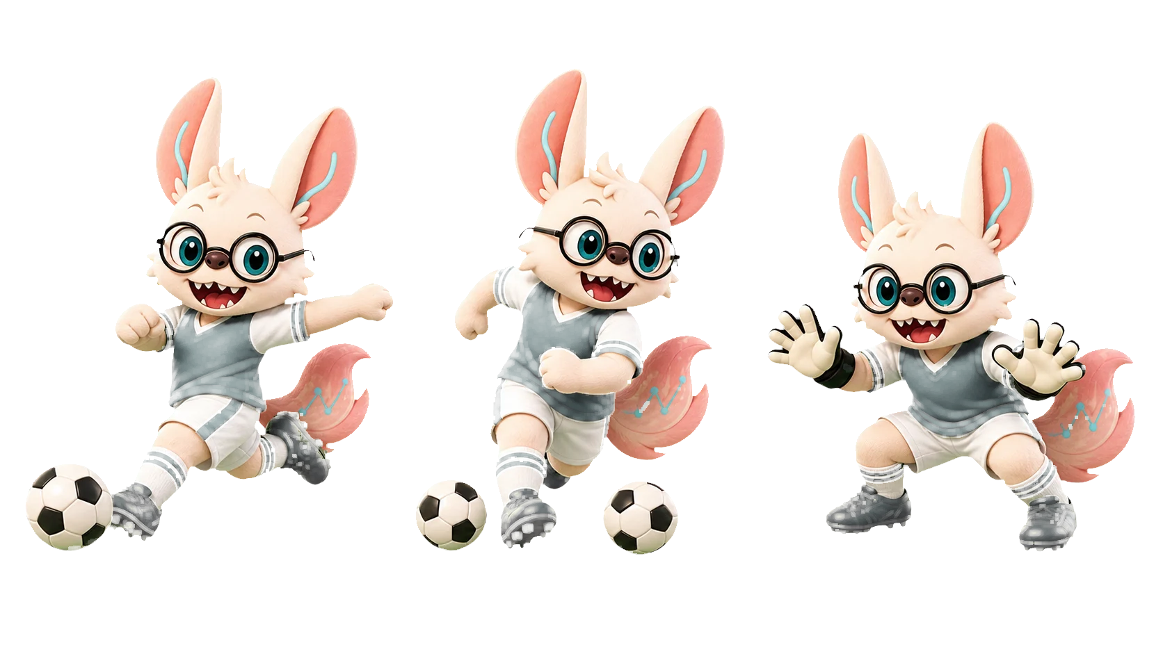
Stars don't win games. Formations do.
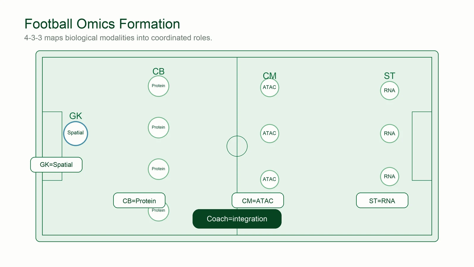
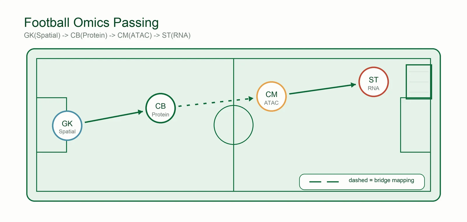
Each omics arrives with its own talent — RNA's speed, ATAC's vision, protein's defense, spatial's positioning. Multi-omics integration is the manager's job: 把十一个天才排成一个阵型 — turn eleven talents into one formation that actually plays together.

Champions Without Stars.
「赢球靠阵型,不靠球星。」
Leicester City, 2015–16: a squad of journeymen, cast-offs and unknowns wins the Premier League at 5000-1 odds — without a single superstar. Six scenes from that season, re-read as multi-omics integration.
The odds nobody believed
Before the season, bookmakers priced a Leicester title at 5000-1 — the same odds as an Elvis sighting. A team with no superstars started winning from day one anyway.
Integration starts here. Not collecting stars, but a formation that already works. See the paradigms ↓
The fastest counter
Eleven straight games with a goal — every time Vardy got the ball it felt like fast-forward, one counter slicing through the whole defensive line.
Transcriptome (scRNA). The fastest, brightest signal on the pitch — but a striker alone never wins a title.
Two lungs, everywhere
The joke went that 71% of Earth is covered by water, and the rest is covered by N'Golo Kanté. He turned up at every duel, stitching defense and attack into one piece.
The midfield is integration itself. The engine that connects every position and lets signals travel. See the methods ↓
The old guard
Two centre-backs in their thirties — no pace, just positioning and cover — cutting off every suspicious pass at the last line.
Protein (CITE-seq). The confirmation layer that settles identity disputes RNA and ATAC argue about.
Position before saves
Schmeichel's numbers were never flashy, but he was already standing in the hardest spot before every shot arrived.
Spatial context. Where a cell sits in the tissue can matter more than how much it expresses. See spatial methods ↓
A different plan for every opponent
Possession one week, counter-attack the next; rotations that changed the shape without breaking it. Ranieri prepared a bespoke answer for every opponent.
Bridge integration. The system adapts — aligning the same team to every new dataset and every new species. See the methods ↓
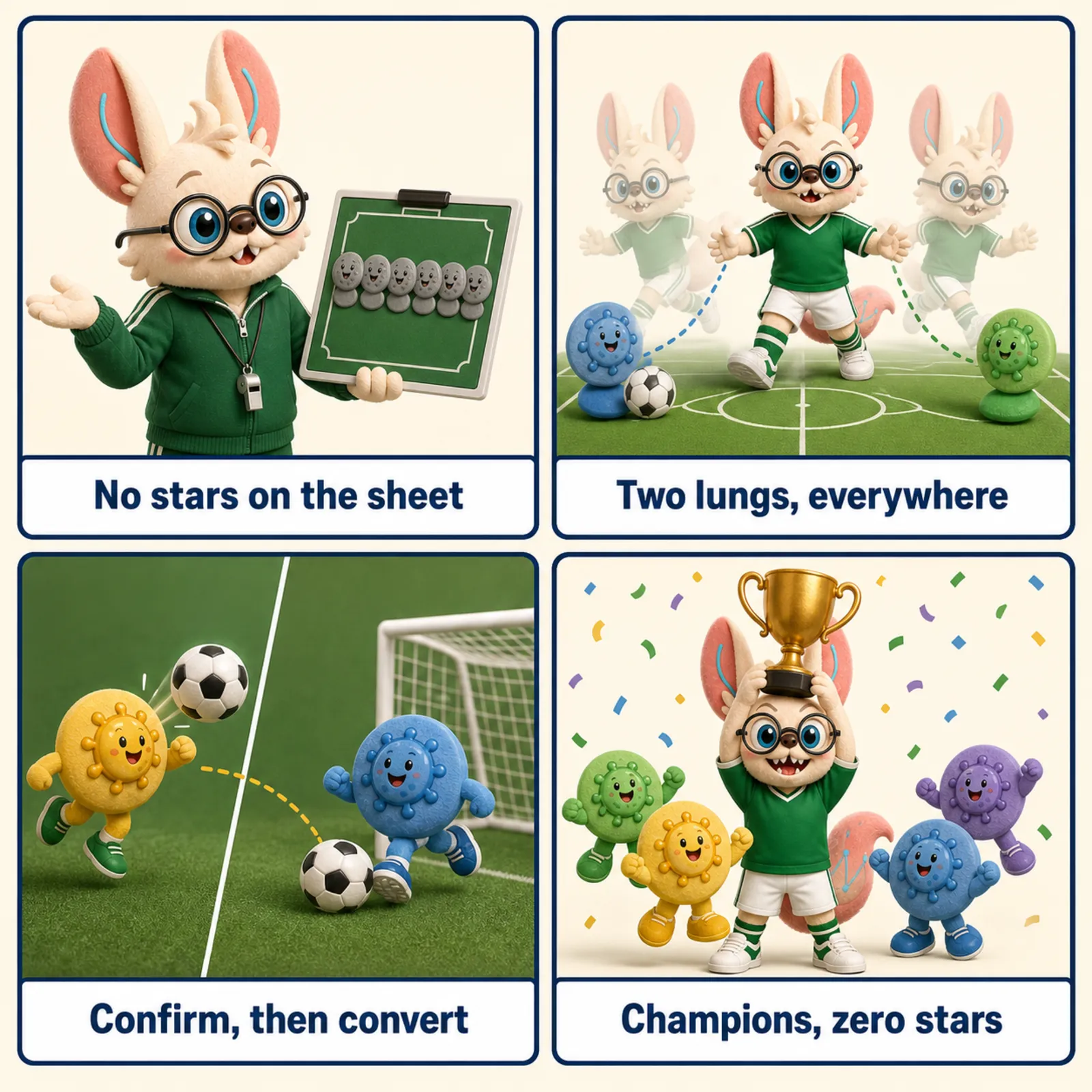
5000-1 的赔率,0 个球星,1 座冠军 —— integration wins games, not any single modality.
📖 What is Single-Cell Multi-Omics Integration?
Single-cell multi-omics integration combines measurements of different molecular layers (transcriptome, epigenome, proteome, spatial location) from the same or related cells to build comprehensive cellular maps. This integration is essential for understanding cell states, developmental trajectories, disease mechanisms, and therapeutic responses.
Why Multi-Omics Integration Matters
- Comprehensive Cell State Definition: Single modalities provide incomplete views; RNA tells what's transcribed, ATAC reveals accessible chromatin, proteins show functional output
- Regulatory Mechanism Discovery: Linking chromatin accessibility → transcription → protein abundance reveals gene regulatory networks and signaling cascades
- Batch Effect Correction: Harmonizing data across experiments, technologies, and labs enables atlas-scale analyses and meta-studies
- Missing Modality Imputation: Predicting unmeasured features (e.g., protein from RNA) reduces experimental costs while maintaining biological insights
- Spatial Context Integration: Combining molecular profiles with spatial locations reveals tissue architecture and cell-cell interactions
- Perturbation Response Modeling: Understanding how genetic or chemical perturbations affect multiple molecular layers simultaneously
⚠️ Integration ≠ batch correction ≠ modality prediction ≠ label transfer
The list above bundles several genuinely different problems under one word. Keeping them apart clarifies what a given method actually does and what output to expect:
- Batch correction — removing technical variation within one modality measured across experiments/labs (Harmony, BBKNN). No second modality involved.
- Modality prediction / imputation — predicting an unmeasured layer from a measured one (e.g. protein from RNA). The output is a synthetic profile, not a joint embedding.
- Label transfer — propagating cell-type annotations from a reference to a query; often a byproduct of integration, not the integration itself.
- Multi-omics integration — combining genuinely different molecular layers from the same or related cells. Its output can be a joint embedding, a joint graph, a cross-modal mapping, an imputed modality, or a set of aligned distributions — the right output depends on the question, not just on the input data.
Integration Paradigms (Fu, Shaliu, et al. Nature Methods, 2025), (Liu, Chunlei, et al. Nature Methods, 2025)
According to the benchmark papers, there are six major multi-omics integration paradigms:
⚠️ Note on Paradigm Classification
The two 2025 benchmark papers formally define four structural paradigms — Vertical, Diagonal, Mosaic, and Cross — based on how modality measurements overlap across cells. Spatial and Perturbation integration, shown as two more panels below, extend that structural taxonomy by data modality type rather than by measurement-overlap structure: a spatial dataset can itself be vertical (paired transcriptome + image at every spot) or mosaic (partial modality coverage across sections), and the same is true for perturbation datasets. The six-panel view below maps common biological use cases; the formal structural taxonomy underneath is the four categories.
🔵 Vertical Integration
🟢 Diagonal Integration
🟡 Mosaic Integration
🔴 Cross Integration
🟣 Spatial Integration
🟠 Perturbation Integration
Each paradigm addresses different data structures and analytical challenges in multi-omics analysis.
📅 Evolution Timeline: From Paired Measurements to Foundation Models
Key Innovations:
- G&T-seq (2015): First simultaneous RNA + DNA methylation
- CITE-seq (2017): RNA + surface protein via antibody tags
- mixOmics (2017): Statistical framework for multi-block data
Era Characteristic: Experimental methods development; simple statistical integration
Key Innovations:
- DIABLO (2019): Multi-omics discriminant analysis
- MOFA+ (2020): Multi-omics factor analysis with covariates
Era Characteristic: Matrix factorization; interpretable latent factors; limited scalability
Key Innovations:
- totalVI (2021): VAE for RNA + protein integration
- Seurat WNN (2021): Weighted nearest neighbor multi-modal analysis
- Concerto (2022): Contrastive learning for 10M+ cells
Era Characteristic: VAE dominance; scalability improvements; atlas-scale analyses
Key Innovations:
- CellOT (2023): Neural optimal transport for perturbations
- SIMBA (2023): Graph embedding with cells + features co-embedded
Era Characteristic: Theoretical rigor; optimal transport theory
Key Innovations:
- scGPT (2024): 100M parameter transformer on 33M cells
Era Characteristic: Pre-training paradigm; 10M+ cell datasets; transfer learning
Key Innovations:
- CellWhisperer (2025): Instruction-tuned multimodal foundation model
- Nicheformer (2025): Spatial multi-omics foundation model
- OmiCLIP (2025): Visual-omics foundation model (H&E + transcriptomics)
- MORPH (2025): Cross-condition perturbation prediction
Era Characteristic: Task-specific foundation models; comprehensive benchmarking; clinical translation focus
Key Directions:
- Unified training APIs: scvi-tools consolidates scVI, totalVI, MultiVI, and scANVI behind one shared training loop, reducing the cost of trying multiple paradigms on the same dataset.
- Pretrained embeddings as integration features: foundation-model embeddings (e.g. Nicheformer, scGPT) are increasingly evaluated as reusable integration features alongside dataset-specific PCA/LSI representations — not as a proven default replacement. Benchmarks (including this hub's own 5-FM comparison) show FM embeddings do not automatically outperform PCA, so the choice remains empirical per dataset/task.
- MOSCOT matures as a general OT backbone: the same optimal-transport framework now spans trajectory, spatial, and cross-modal matching tasks that previously needed separate tools.
- Unified multi-modal containers: MuData and spatialdata converge toward a stable on-disk format spanning RNA+ATAC+protein+spatial in one structure.
Era Characteristic: Consolidation around shared APIs and pretrained scaffolds rather than one-off bespoke integration models per dataset.
🔬 Method Taxonomy: Algorithmic Approaches
By Computational Framework
🧠 Variational Autoencoders (VAE-based)
Principle: Learn probabilistic latent representations with encoder-decoder architecture
Advantages: Uncertainty quantification; generative modeling; missing data imputation
🔄 Contrastive Learning
Principle: Learn representations by pulling similar samples together, pushing dissimilar apart
Advantages: Scalability to millions of cells; no explicit pairing needed; robust embeddings
📊 Graph Neural Networks (GNN)
Principle: Model cells as graph nodes; aggregate information from neighborhoods
Advantages: Captures cell-cell relationships; flexible message passing; spatial awareness
🚀 Optimal Transport
Principle: Find minimal-cost mapping between cell distributions
Advantages: Theoretical guarantees; preserves distributional structure; interpretable
🤖 Foundation Models (Transformers)
Principle: Pre-train large models on massive datasets; fine-tune for specific tasks
Advantages: Transfer learning; few-shot adaptation; generalizable representations
🔗 Matrix Factorization & Classical
Principle: Decompose data matrices into latent factor representations
Advantages: Interpretable factors; computationally efficient; well-understood theory
By Computational Profile
Computational Profile, Not a Fixed Capacity Ceiling
Cell-count tiers below are approximate, reported orders of magnitude from published benchmarks — not an inherent capacity of the method. Actual scaling depends heavily on feature count, GPU/RAM available, batch size, and implementation details. A more useful lens is each method's computational profile:
- CPU-only, no training (MOFA+, DIABLO, mixOmics): factorization on the full matrix; comfortable to ~10K cells on a laptop, but memory-bound as feature count grows.
- Trainable, CPU or single GPU (Seurat WNN, totalVI, MultiVI): WNN needs no GPU; totalVI/MultiVI train faster on GPU but run on CPU too — reported comfortably to ~10K–100K cells.
- GPU-preferred, mini-batch training (Concerto, SIMBA, scBridge): scales sublinearly via mini-batching; reported to ~100K–1M cells given sufficient GPU memory.
- Pretrained + fine-tune/inference only (foundation models: scGPT, CellWhisperer, Nicheformer): the expensive step (pretraining on >1M cells) is amortized once; per-dataset inference/fine-tuning cost is what actually matters for a new project, and out-of-sample mapping (no retraining needed) is often the bigger practical advantage than raw cell count.
- Scalable specialized algorithms, not pretrained (SnapATAC2, SIMBA): no pretraining step — these are trained fresh per dataset, but engineered (efficient data structures, GPU-accelerated linear algebra) to scale to atlas-size inputs directly; don't confuse "handles >1M cells" with "foundation model."
📄 Landmark Papers by Computational Framework (2015-2025)
🧬 Experimental Technologies (Foundation)
CITE-seq: Simultaneous epitope and transcriptome measurement in single cells
- Antibody-oligonucleotide conjugation method
- Validated on PBMC immune cell populations
- Foundation for multi-modal single-cell biology
scONE-seq: A single-cell multi-omics method enables simultaneous dissection of phenotype and genotype heterogeneity from frozen tumors
- Works with frozen tissue samples
- Simultaneous DNA and RNA profiling
- Tumor heterogeneity analysis
🔷 Variational Autoencoders & Probabilistic Models
Joint probabilistic modeling of single-cell multi-omic data with totalVI
- Batch correction across technologies
- Protein imputation from RNA
- Uncertainty quantification
MultiVI: deep generative model for the integration of multimodal data
- Handles paired and unpaired RNA + ATAC measurements, including mosaic datasets with missing modalities
- Missing modality imputation
- Joint latent representation and modality-specific generation for RNA + ATAC
Cobolt: integrative analysis of multimodal single-cell sequencing data
- Hierarchical latent variable model
- Handles incomplete modality measurements
- Supports SNARE-seq and other multimodal data
Multigrate: single-cell multi-omic data integration
- Multi-view VAE supporting RNA+ADT+ATAC combinations, not tied to one specific assay pairing
- Transfer learning maps a new query dataset into an existing reference atlas without retraining
- Compares favorably to data-specific methods on both integration and imputation
🕸️ Graph-Based Methods
Integrated analysis of multimodal single-cell data (Seurat WNN)
- Cell-specific modality weighting
- Works with RNA+ADT, RNA+ATAC
- Integrated into widely-used Seurat package
SIMBA: single-cell embedding along with features
- Unified cell-feature embedding space
- Multi-omics native support
- Scales to 1.3M cells in 1.5 hours
Multi-omics single-cell data integration and regulatory inference with graph-linked embedding
- Diagonal (unpaired) integration of scRNA-seq and scATAC-seq via a graph variational autoencoder
- Embeds a prior knowledge graph (gene-to-peak regulatory links) directly into the alignment objective
- Jointly infers a regulatory graph as a byproduct of integration, not just a shared embedding
- Reports among the strongest batch-correction performance in independent diagonal-integration benchmarks
🔄 Optimal Transport Methods
Learning single-cell perturbation responses using neural optimal transport (CellOT)
- Drug response prediction
- Genetic knockout effects
- Cross-patient generalization
Cross-modality matching and prediction of perturbation responses with labeled Gromov-Wasserstein optimal transport
- Incorporates perturbation labels
- RNA → protein prediction
- Dose-response preservation
SCOT: Single-Cell Multi-Omics Alignment with Optimal Transport
- Aligns modalities using only within-modality distance structure, not cross-modality feature correspondence
- Fully unsupervised — no labeled anchors or paired cells required
- Competitive with supervised alignment methods on real multi-omics benchmarks
Mapping cells through time and space with moscot
- Low-rank entropic (Gromov-)Wasserstein solvers with linear time/memory complexity
- One framework spans temporal, spatial, and cross-modality matching problems instead of separate tools per task
- Unbalanced formulations model cell proliferation/death during matching
- Demonstrated reconstructing 1.7M-cell, 20-timepoint mouse embryo development
🧠 Deep Learning & Neural Networks
Deep learning and alignment of spatially resolved single-cell transcriptomes with Tangram
- Works with any spatial technology (MERFISH, Visium, smFISH)
- Expands gene coverage to genome-wide scale
- Automated histological registration module
scJoint integrates atlas-scale single-cell RNA-seq and ATAC-seq data with transfer learning
- Processes 1M+ cells in 2 hours
- 84% label transfer accuracy
- Effective batch correction across platforms
scBridge embraces cell heterogeneity in single-cell RNA-seq and ATAC-seq data integration
- Progressive integration strategy
- Exploits cell heterogeneity as advantage
- Superior performance on challenging datasets
scMODAL: a general deep learning framework for comprehensive single-cell multi-omics data alignment with feature links
- GAN-based architecture for alignment
- Works with limited feature correlations (e.g., gene-protein pairs)
- Cross-modality imputation and prediction: 29-34% imputation improvement
- Demonstrated on CITE-seq + CyTOF integration
A visual-omics foundation model to bridge histopathology with spatial transcriptomics (OmiCLIP)
- Image → transcriptomics prediction
- Tissue section alignment
- Cell type annotation from H&E
- Spatial decomposition
🎯 Contrastive Learning
Contrastive learning enables rapid mapping to multimodal single-cell atlas of multimillion scale (Concerto)
- 10M cell reference atlas in 1.5 hours
- Query mapping in 8 seconds (10K cells)
- Superior clustering and classification
🤖 Foundation Models & Transformers
scGPT: toward building a foundation model for single-cell multi-omics using generative AI
- Cell type annotation
- Batch correction
- Perturbation prediction
- Gene network inference
Multimodal learning enables chat-based exploration of single-cell data (CellWhisperer)
- Natural language biological queries
- Multi-task learning (classification, clustering, prediction)
- Zero-shot generalization
Nicheformer: a foundation model for single-cell and spatial omics
- Joint pretraining on 57M dissociated + 53M spatial cells (110M+ total)
- Technology-aware rank tokens and contextual <ORGANISM>/<ASSAY>/<MODALITY> tokens
- Transfers spatial niche labels back onto dissociated scRNA-seq with no spatial measurement needed at query time
- Zero-shot niche and cell-type annotation across tissues without retraining
🌉 Mosaic & Bridge Integration
Stabilized mosaic single-cell data integration using unshared features (StabMap)
- Multi-hop integration without direct feature overlap
- Leverages non-overlapping features
- Supports supervised and unsupervised modes
Building a cross-species cell atlas with interpretable deep learning (Dictionary Learning)
- Human-mouse integration
- Cross-platform harmonization
- Conserved program discovery
🔬 Perturbation & Response Prediction
Predicting cell morphological responses to perturbations using generative modeling (IMPA)
- Drug response prediction from imaging
- Handles batch effects in HCS
- Generative modeling for perturbation screens
📊 Benchmark & Review Papers
Multitask benchmarking of single-cell multimodal omics integration methods
- No universal winner; task-dependent performance
- Deep learning dominates diagonal/cross integration
- Batch correction often trades off with biological preservation
Benchmarking single-cell multi-modal data integrations
- Multi-gradient AUC for robustness
- Hardware scalability testing (500GB RAM, 24h limits)
- Cross-modality imputation assessment
How to build the virtual cell with artificial intelligence: Priorities and opportunities (AIVC)
- Universal representations (URs) across scales
- Virtual instruments (manipulators & decoders)
- Foundation model architecture for cells
The Human Cell Atlas: from a cell census to a unified foundation model
🔧 Methods Development & Innovation
SnapATAC2: A fast, scalable and versatile tool for analysis of single-cell omics data
- O(n) complexity vs O(n²) for competitors
- 63.4% cost reduction vs ArchR
- 200K cells in 13.4 minutes
SIMVI disentangles intrinsic and spatial-induced cellular states in spatial omics data
- Asymmetric regularization for identifiability
- Single-cell spatial effect estimation
- Causal inference integration (DML)
MORPH predicts the single-cell outcome of genetic perturbations across conditions and data modalities
- Cross-cell line transfer learning
- Combinatorial perturbation modeling
- Active learning for experiment design
MetaQ: fast, scalable and accurate metacell inference via single-cell quantization
- 100K cells in 0.3h vs 26.7h (SEACell)
- 88% balanced accuracy vs 84% (baseline)
- Native multi-omics support
ADTnorm: robust integration of single-cell protein measurement across CITE-seq datasets
- Cross-institutional integration
- Antibody titration optimization
- Auto-gating (80-100% accuracy)
📚 Comprehensive Method Comparison
By Integration Category & Performance
| Method | Year | Category | Modalities | Scale | Key Strength |
|---|---|---|---|---|---|
| Vertical Integration (Paired Multi-Modal) | |||||
| Seurat WNN | 2021 | Vertical | RNA+ADT, RNA+ATAC | ~100K cells | Cell-specific modality weighting; widely adopted |
| totalVI | 2021 | Vertical/Cross | RNA+ADT | ~50K cells | Probabilistic; batch correction; imputation |
| Multigrate | 2022 | Vertical/Cross | RNA+ADT+ATAC | ~100K cells | Tri-modal support; transfer learning onto reference atlases |
| Diagonal Integration (Unpaired, Non-Overlapping) | |||||
| scBridge | 2023 | Diagonal | RNA+ATAC | ~50K cells | Superior dimensionality reduction & clustering |
| GLUE | 2022 | Diagonal | RNA+ATAC | ~50K cells | Graph neural network; best batch correction |
| scJoint | 2022 | Diagonal | RNA+ATAC | ~100K cells | Multi-batch integration; transfer learning |
| SCOT | 2022 | Diagonal | Any unpaired | ~10K cells | Gromov-Wasserstein OT; no correspondence needed |
| Mosaic Integration (Overlapping Incomplete) | |||||
| StabMap | 2023 | Mosaic | Any combination | ~50K cells | Flexible; efficient; handles any modality pattern |
| MultiVI | 2023 | Mosaic | RNA+ATAC (paired or unpaired) | ~100K cells | VAE-based; missing modality imputation |
| Cobolt | 2021 | Mosaic | RNA+ADT+ATAC | ~50K cells | Bayesian framework; uncertainty quantification |
| Spatial Integration | |||||
| SIMVI | 2025 | Spatial | Spatial transcriptomics | ~60K cells | Disentangles intrinsic vs spatial variation |
| OmiCLIP | 2025 | Spatial | H&E + ST | 2.2M pairs | Visual-omics foundation model; H&E → gene expression |
| Tangram | 2021 | Spatial | Spatial mapping | ~50K cells | Maps scRNA-seq to spatial coordinates |
| Nicheformer | 2025 | Spatial | Spatial + scRNA-seq | 110M+ cells | Foundation model; zero-shot niche annotation transfer |
| MOSCOT | 2025 | Cross/Spatial | Any + time/space | 1.7M+ cells | Unified OT for trajectory + spatial + cross-modal mapping |
| Perturbation-Aware Integration | |||||
| CellOT | 2023 | Perturbation | RNA-seq (protein/imaging) | ~50K cells | Neural OT; single-cell predictions |
| MORPH | 2025 | Perturbation | RNA + Imaging | ~300K cells | Cross-modality; cross-cell line transfer |
| Labeled GWOT | 2025 | Perturbation | RNA + Protein | ~50K cells | Label-constrained OT; L-fold speedup |
| Classical/Statistical Methods | |||||
| MOFA+ | 2020 | Vertical | Any | ~10K cells | Interpretable factors; handles covariates |
| mixOmics | 2017 | Vertical | Any | ~5K cells | Multiblock projection to latent structure (PLS); statistical rigor |
🎯 From Scientific Question to Method
34 landmark papers are a lot to hold at once. The table below compresses them back into the question that actually matters when starting a project: what am I asking, what object do I need as output, and which approach typically produces it?
| Scientific question | Desired output object | Typical approach |
|---|---|---|
| Same CITE-seq cell — RNA + ADT should jointly define cell state | Weighted joint neighbor graph | WNN |
| RNA + ADT, but protein has ambient background needing denoising | Probabilistic joint latent | totalVI |
| RNA/ATAC partially paired — some cells missing one modality | Joint latent + per-cell imputation | MultiVI (mosaic) |
| RNA and ATAC measured in genuinely different cells, no shared modality | Cross-modal alignment | GLUE / SCOT / related (diagonal) |
| Map dissociated scRNA-seq cells onto a tissue section | Cell → space mapping | Tangram / optimal-transport approaches |
| Perturbation response with no cell-level correspondence before/after | Distribution-to-distribution mapping | CellOT / optimal transport |
| Just need RNA differential expression | No joint integration needed | Modality-specific statistical model (see "When not to integrate" below) |
💡 Practical Implementation Guide
Choosing the Right Method: Decision Framework
Step 1: Identify Your Data Structure
The real question isn't "is there more than one batch" — it's cell correspondence (are modalities measured on the same cells?) crossed with modality/feature overlap (do datasets share modalities, features, or a bridge?).
- Are modalities measured on the same cells?
- Yes, in every cell → Vertical integration (paired)
- Yes, in some cells / some modalities missing per cell → Mosaic integration
- No — different cells per modality, no shared modality → Diagonal integration (aligned via shared features/cell types or a bridge dataset)
- All modalities present in every batch, but multiple batches/labs with technical variation? → Cross integration. Per Liu et al. (2025)'s formal definition, this is the case where "all data modalities are present in each of all batches in a dataset" — it is not the same as single-modality batch correction (see the box above): the method must remove technical variation from the joint multi-modal profile while keeping the cross-modal relationships within each cell intact, not just align one modality's embedding.
- Spatial data? → Spatial methods — itself vertical (paired profile + coordinate at every spot) or mosaic (partial modality coverage across sections)
- Perturbation data? → Perturbation-aware — check cell correspondence across conditions the same way (paired before/after vs. unpaired distributions)
Step 2: Consider Your Computational Resources
Limited Resources (no GPU, <32GB RAM):
- Classical methods
Moderate Resources (GPU optional, 32-64GB RAM):
- Most VAE-based and graph methods
High-End Resources (GPU required, 64GB+ RAM):
- Foundation models
Common Pitfalls & Best Practices
🚫 When not to integrate
Do not integrate merely to obtain a prettier UMAP. If the actual goal is modality-specific differential expression (RNA DE), differential accessibility (ATAC DA), or any per-modality statistical test, keep the original modality-specific count data and statistical model — a joint latent space or joint graph is the wrong tool for that question and can bias the test. Joint embeddings/graphs earn their place for representation learning, clustering, cell-type annotation, and cross-modality matching — not as a default preprocessing step for every downstream analysis.
- Data Quality First: Ensure appropriate cell calling, modality-specific QC, doublet handling, and contamination assessment before integration — avoid universal hard thresholds; QC cutoffs should reflect assay, sequencing depth, and dataset structure. Use standard pipelines (Scanpy, Seurat). Bad data → bad integration.
- Modality- and model-specific preprocessing: RNA, ATAC, and protein have different measurement distributions, and preprocessing must match both the assay and the downstream model. For example, WNN commonly uses log-normalized RNA, TF-IDF/LSI for ATAC, and CLR/DSB for ADT, whereas generative models such as totalVI/MultiVI expect their own specified count-level inputs rather than those pre-derived features.
- Evaluation Metrics Matter: Use multiple complementary metrics (ARI, NMI, ASW for clustering; kBET, iLISI for batch mixing). Single metrics can be misleading.
- Batch Effect vs Biological Variation: Over-correction removes biology; under-correction leaves technical artifacts. Check cell type separation alongside batch mixing.
- Held-Out Testing: Evaluate on held-out batches or cell types, not just held-out cells from training conditions. Tests true generalization.
- Baseline Comparisons: Always compare against simple baselines (PCA, naive concatenation, per-modality analysis). Complex methods should outperform simple ones.
- Computational Scalability: Test methods on your actual data size. Many methods fail silently or degrade performance on large datasets.
- Biological Validation: Computational integration should reveal biologically meaningful patterns. Validate key findings with marker genes, known cell types, or experimental follow-up.
- Hyperparameter Tuning: Default parameters often suboptimal. Use cross-validation or grid search for critical parameters (latent dimensions, regularization, learning rate).
- Reproducibility: Report random seeds, package versions, preprocessing steps, and hyperparameters. Provide code and (when possible) data.
Software Ecosystem & Tools
- Scanpy: Standard Python toolkit for preprocessing, analysis, visualization. Foundation for many integration methods.
- Seurat: R package with Seurat v3/v5 integration, WNN, UMAP. Industry standard for single-cell RNA-seq.
- scvi-tools: PyTorch-based framework for probabilistic models (scVI, totalVI, MultiVI, scANVI). GPU-accelerated.
- Muon: Python package for multimodal omics analysis. Integrates with Scanpy ecosystem.
- LIGER: R package for integrative non-negative matrix factorization. Good for cross-platform integration.
- Harmony: Fast batch correction algorithm. Works on PCA embeddings. Widely used for large-scale integration.
- ArchR: R package for scATAC-seq analysis (2021, Nat Genetics) — Seurat's epigenomic companion for peak calling, gene-score computation, and downstream integration with RNA.
- Pertpy: Python framework unifying perturbation analysis workflows (CPA, GEARS, and optimal-transport methods like CellOT behind one interface with standard evaluation metrics).
-
MuData (2022, Genome Biology):
The stable multi-modal AnnData container — paired modalities stored in one
.h5mufile with linkedobs/var, the format Muon (above) is built on. - spatialdata (2024, Nat Methods): OME-Zarr-based container unifying points, polygons, images, and tables for spatial multi-omics across platforms.
⚖️ Side-by-Side: Combining Modalities — Weighted-Graph (WNN) vs Joint Generative (totalVI / MultiVI)
When RNA and a second modality (protein in CITE-seq, chromatin in 10x Multiome) are measured in the same cell, the integration question is when to combine them: fuse per-modality neighbor graphs after embedding each separately (WNN), or learn a single joint latent space from the raw counts of both (a joint VAE like totalVI / MultiVI)?
The same paired cells become one integrated representation in two different ways, depending on whether modalities are fused late (graph) or early (latent):
The root decision is fuse graphs after separate embeddings vs learn one joint latent from raw counts. WNN is non-generative and hands you an interpretable per-cell weight showing which modality drives each cell, but it does no denoising or imputation; totalVI/MultiVI is probabilistic — it denoises, imputes missing modalities, and corrects batch — at the cost of training a model. WNN and totalVI both assume paired cells (the same cell measured in every modality). MultiVI generalizes beyond the fully paired case: some cells may have RNA only, some ATAC only, and some both — it natively handles paired, unpaired, or mixed modality availability (mosaic integration), and can infer/impute the unobserved RNA or ATAC modality within its supported RNA–ATAC setting. For fully diagonal data (no cell overlap and no shared modality at all) you still need anchor transfer, GLUE, or LIGER.
🛠️ Hands-On Practice
The steps below walk through the joint-VAE route on CITE-seq with totalVI — one shared latent from RNA + protein — and note the WNN (graph) alternative and the MultiVI variant for RNA + ATAC.
Environment & packages
scvi-tools provides totalVI/MultiVI; scanpy/muon/mudata hold the modalities and run the WNN graph route in Python (Seurat's WNN is the R equivalent).
conda create -n multiomics python=3.10 -y
conda activate multiomics
pip install scvi-tools scanpy muon mudata
# WNN graph route is in muon (Python) or Seurat (R)
Hardware. WNN runs on a laptop; totalVI/MultiVI training wants a GPU (minutes) but works on CPU (slower) for datasets up to ~100k cells.
Data structures & formats
- CITE-seq
AnnData— RNA counts inadata.X, protein (ADT) counts inadata.obsm["protein_counts"] - 10x Multiome
MuData—mdata["rna"](genes) +mdata["atac"](peaks), the same cells in both - Pairing requirement varies by method — WNN and totalVI need the same cells measured in every modality (paired). MultiVI is designed for mosaic RNA/ATAC data — paired, unpaired, or a mix of RNA/ATAC availability across cells — and can infer/impute the unobserved RNA or ATAC modality within that supported RNA–ATAC setting.
- Joint latent — written to
adata.obsm["X_totalVI"]/["X_multivi"]for neighbors + UMAP - Batch key —
adata.obs["batch"](donor / lane) for the model to correct
Minimal code walkthrough
Fit totalVI on CITE-seq to get one joint latent from RNA + protein.
import scvi, scanpy as sc

# CITE-seq: RNA counts in adata.X, protein (ADT) counts in adata.obsm["protein_counts"]
adata = sc.read_h5ad("cite_seq.h5ad")

# totalVI jointly models RNA (negative binomial) and protein (with ambient background)
scvi.model.TOTALVI.setup_anndata(
    adata,
    protein_expression_obsm_key="protein_counts",
    batch_key="batch",
)
model = scvi.model.TOTALVI(adata)
model.train()

# One joint latent from BOTH modalities; denoised protein is available too
adata.obsm["X_totalVI"] = model.get_latent_representation()
sc.pp.neighbors(adata, use_rep="X_totalVI"); sc.tl.umap(adata)
Swap in the graph route, or MultiVI for RNA + ATAC:
# Graph-level alternative — WNN via muon (Python port of Seurat's WNN):
# import muon as mu
# mu.pp.neighbors(mdata)        # per-modality graphs -> one weighted joint graph
# mu.tl.umap(mdata)

# RNA + ATAC (10x Multiome) instead of CITE-seq -> MultiVI:
# amvi = scvi.data.organize_multiome_anndatas(adata_paired, adata_rna, adata_atac)
# MultiVI's batch_key must hold the modality-availability label ("paired"/"expression"/"accessibility")
# added by organize_multiome_anndatas -- this is required by the model's architecture, not a
# stand-in for donor/lane batch. Real technical batch goes in categorical_covariate_keys instead:
# scvi.model.MULTIVI.setup_anndata(amvi, batch_key="modality", categorical_covariate_keys=["donor"])
# mvi = scvi.model.MULTIVI(amvi, n_genes=n_g, n_regions=n_r); mvi.train()
Common pitfalls & tips
- Paired vs mosaic vs diagonal. WNN and totalVI require the same cells in every modality. MultiVI is built for mosaic data — paired, unpaired, or mixed RNA/ATAC availability across cells — so it does not require full pairing. For fully diagonal data (no cell overlap, no shared modality at all) use Seurat anchor transfer, GLUE, or LIGER instead.
- Never concatenate raw features and PCA. RNA counts, protein ADT, and sparse binary ATAC peaks live on wildly different scales — naive concatenation lets one modality dominate the embedding.
- Protein has ambient background. ADT counts include background binding; totalVI models it explicitly, so don't preprocess protein like RNA (use CLR for WNN, raw counts for totalVI).
- ATAC preprocessing is model-specific. The classical WNN/LSI pipeline needs peak calling then TF-IDF/binarization before use. Generative models have their own input contract instead: MultiVI takes ATAC as its own count/binary-accessibility likelihood term and should not be fed pre-computed LSI/TF-IDF features meant for the WNN route — check what each model expects rather than assuming one preprocessing recipe fits all.
- Modality-availability label vs. technical batch are not the same. For MultiVI,
batch_keymust hold the modality-availability indicator (paired/expression/accessibility) — that's required by the model's architecture, not a stand-in for donor/lane batch. Pass real technical batch effects viacategorical_covariate_keysinstead, so both are corrected. - Inspect the WNN weights. The per-cell modality weights are interpretable; a modality with no signal in some cells should get a low weight — check them to catch a broken or empty modality.