Tokenization Strategies
Translating Biology into AI-Readable Language
Understanding how biological data is converted into tokens is fundamental to building effective foundation models. This guide explores the major tokenization strategies used in single-cell multi-omics, protein modeling, and DNA sequence analysis, using intuitive LEGO analogies to make these concepts accessible.
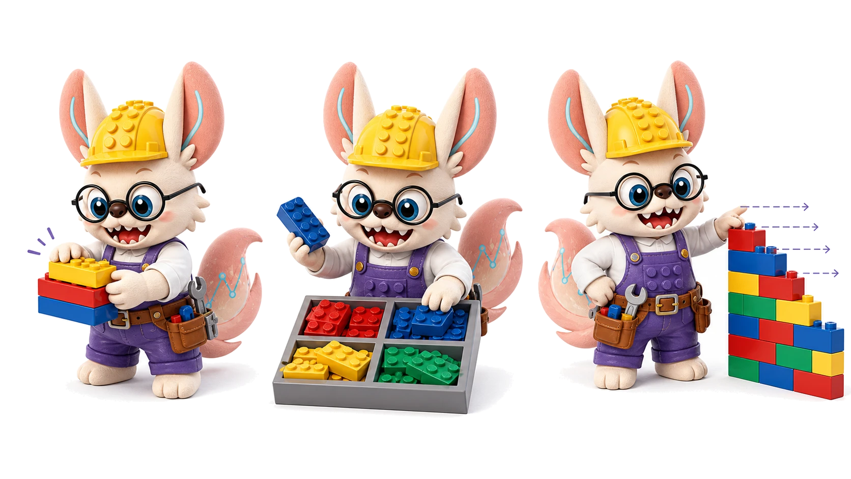
No castle without a parts list.
Every LEGO castle begins before the first brick snaps in — with someone deciding which pieces exist and in what order. Tokenization is that decision for AI: how a messy bucket of biology becomes a neat line of parts a model can build with.

Split, Then Snap.
「先分件,再拼装。」— Every LEGO build starts with sorting the bucket.
No builder dumps the bucket straight onto the table and hopes for a castle. You sort first: decide which units exist, in what order, at what size. Tokenization is exactly that sorting step for AI — six scenes from the workbench, re-read as tokenization strategies.
No build without a plan
Every LEGO set opens with the instruction booklet: before a single brick is placed, someone has already decided which pieces exist and in what order they connect.
Tokenization itself. The plan that turns a messy bucket into a buildable sequence — without it, the model has a pile, not a project.
Three bricks, one click
Three small bricks click together and hold as one larger piece. The wall no longer cares about the three — only about the unit they became.
Codon-level tokenization. Three nucleotides snapped as one codon, read as a single functional unit. See the codon strategy ↓
Pick from the tray, don't mold new bricks
A master builder rarely molds custom pieces. They reach into the sorting tray and reuse the common bricks that fit everywhere — cheaper, faster, and the castle stands the same.
BPE / subword units. Don't mint a token for every word; pick the frequent reusable pieces already lying in the corpus. See BPE ↓
The wrong page of instructions
You follow the booklet faithfully, step by step — but it is the page from a different set. Every brick clicks perfectly, and the wrong castle rises anyway.
Garbage tokens in, garbage out. A wrongly segmented unit poisons everything downstream — tokenize wrong, and the model builds confidently on a false plan.
A wall laid with offset bricks
Each course overlaps the last by half a brick: stronger than stacked columns — but you spend far more bricks to cover the same wall.
K-mer tokenization. Overlapping windows chained across the sequence: continuous coverage, redundancy that burns budget. See k-mer ↓
When a piece is missing
One big custom piece missing stops the whole build. The tiniest universal brick is never out of stock — slow, but it always fits.
Byte-level tokenization. The smallest unit never goes OOV: full coverage and zero missing pieces, at the price of very long builds. See trade-offs ↓
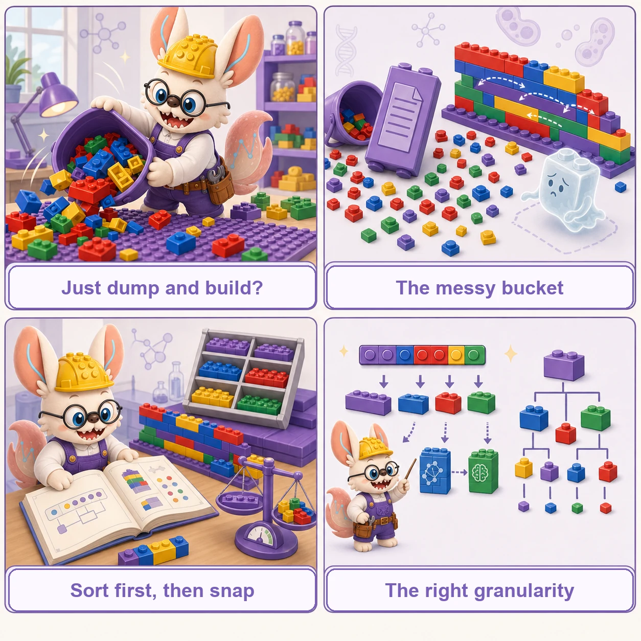
按任务选套装:没有最好的粒度,只有合适的套装 —— the right tokenization is the set your task can build with.
The Problem: Biology is Messy, AI Needs Order
The LEGO Analogy: Imagine a single cell as a giant bucket full of unsorted LEGO bricks.
Each type of brick (color/shape) represents a different Gene.
The number of bricks of that specific type represents its Expression Level (how active that gene is).
An AI model (like a Transformer) is a master builder, but it can't just grab a handful from the messy bucket. It needs the bricks sorted, labeled, and handed to it in a specific sequence. Tokenization is the process of organizing that messy bucket into a neat line of inputs the builder can use.
Depending on what we want the model to learn, we use different strategies to sort and present these "bricks".
Visual Guide to Core Tokenization Concepts
Before diving into the details, let's understand the core concepts visually using our LEGO analogy.
Navigation Map — 12 Strategies, 4 Biological Domains
These strategies answer different questions depending on what type of data you're working with. The LEGO analogy stays the same — what changes is which property of the brick matters.
| Domain | Strategy | The core question | Models |
|---|---|---|---|
| scRNA-seq Gene expression in single cells | The Basics | How do I combine gene identity + expression value into one token? | — |
| Rank-Based | Which genes are relatively more active? (ignore absolute counts) | Geneformer, iSEEEK | |
| Expression Binning | Which expression level category is this gene in? | scGPT, scBERT | |
| Read-Depth-Aware | What would expression look like at full sequencing depth? | scFoundation, AIDO.Cell | |
| Cell2Sentence | Can I turn cell data into a plain text sentence for a standard LLM? | C2S-Scale (27B) | |
| DNA / Genomics Nucleotide sequences | K-mer | What are the overlapping short motifs in this sequence? | DNABERT, Nucleotide Transformer |
| BPE + IUPAC | How do I encode personal diploid variants efficiently? | VariantFormer | |
| Codon-Level | Does the specific triplet (not just the amino acid) matter? | CodonFM, EnCodon | |
| Single-Nucleotide + SSM | Can I skip k-mer vocabulary entirely and scan 1M+ bp in linear time? | HyenaDNA, Evo, Evo 2 | |
| ATAC-seq / Chromatin Open chromatin | Genome Coordinates | Where on the genome is this accessible region? (location = identity) | ChromFound |
| Protein Amino acid sequences | Amino Acid | Which of the 20 building blocks is at each position? | ESM3, ProGen2 |
| Cross-species Multi-organism integration | Macrogene | Can I group orthologous genes across species into one shared token? | SATURN |
The Basics: Identity & Count
A token is a single unit of information for the model. In single-cell data, we usually need two pieces of information combined:
- What is it? (The Gene Identity, e.g., "TP53" or a red brick).
- How much? (The Expression Value, e.g., "50 counts" or a stack of 50 bricks).
The challenge is how to combine these two very different types of information into a single vector representing the token.
Strategy: Rank-Based Tokenization
The Problem: Sometimes we have "technical noise" (batch effects). One experiment might yield giant stacks of bricks (high sequencing depth), and another yields tiny stacks, even for the same biological cell type.
The Solution: Ignore the exact height. Just line them up from tallest to shortest. As long as the relative order is preserved (Red is taller than Blue), the resulting sequence of tokens is the same, making the model immune to batch differences in sequencing depth.
| Full rank | All expressed genes ranked, sequence length = # genes expressed in that cell |
| Top-N truncated | Only top N genes kept (e.g. N≈2,048) to fit a fixed context window — Geneformer default |
| Fails when: | Many genes tie at zero counts — rank order among the unexpressed tail is arbitrary and adds noise, not signal. |
Strategy: Expression Binning
The Problem: Standard language models work best with a fixed dictionary of words (categorical data). Actual expression counts are continuous numbers (1, 2, 50, 1000...).
The Solution: We create buckets (bins) for different ranges of heights. Instead of saying "Height 45", we throw it into the "Medium Height Bucket". Now, the token isn't a number, it's a category: [GeneID] + [MediumBin].
| Equal-width bins | Fixed count ranges (e.g. 0–20, 21–80, 81+) — simple, but bins can be very imbalanced in size |
| Equal-frequency (quantile) bins | Each bin holds the same number of genes — scGPT's default, ~51 bins |
| Fails when: | Bin edges fit on one dataset don't transfer cleanly to a batch with a different expression distribution — genes get mis-binned under domain shift. |
Strategy: Read-Depth-Aware (RDA) Tokenization
The Problem: Different cells have different sequencing depths—some have 10,000 total counts, others only 1,000. This makes expression values hard to compare directly.
The Solution: Keep the continuous expression values (don't discretize!), but add special "depth tokens" that tell the model: "This cell was supposed to have T=10,000 counts, but we only sampled S=1,000." The model learns to mentally "scale up" the values during pretraining.
Key Benefit: Enables expression enhancement—the model can predict what gene expression would look like at higher sequencing depth, effectively denoising sparse data.
| T token | Target/original total UMI count the cell was meant to have |
| S token | Sampled/observed total UMI count actually sequenced |
| Fails when: | Sampled depth S is extremely low (heavy dropout) — the T/S ratio the model must invert becomes unreliable when there's almost nothing to scale up from. |
Strategy: Cell2Sentence (C2S)
The Idea: Instead of stacking bricks to show expression level, lay them out in a horizontal line. High expression? Repeat that brick many times. Low expression? Just one or two repeats.
Why It Matters: This transforms cell data into text-like "sentences" that standard large language models (GPT, LLaMA) can understand. You can even ask natural language questions about cells!
| Repeat encoding | Gene token repeated proportional to (rank-transformed) expression count |
| Context cap | Max repeats / sequence-length truncation — controls how much the "sentence" can grow |
| Fails when: | A handful of highly expressed housekeeping genes can dominate the token budget, crowding out rare but biologically important marker genes. |
Choosing Among the 4 scRNA Tokenization Strategies
All four apply to scRNA-seq data. What they preserve — and sacrifice — is different.
| Strategy | Absolute counts preserved? | Batch / depth robust? | Sequence length | Works with standard LLMs? | Best when… |
|---|---|---|---|---|---|
| Rank-Based | ✗ (discarded) | ✓✓ (best) | = # expressed genes | ✓ (integer position) | Cross-batch cell-type classification; depth varies wildly across batches |
| Binning | Partial (quantized) | ✓ (quantization absorbs depth noise) | = # expressed genes | ✓ (categorical token) | Moderate depth variation; need to retain some expression magnitude |
| Read-Depth-Aware | ✓✓ (continuous) | ✓ (via depth tokens T, S) | = # expressed genes + 2 | Needs custom embedding | Expression enhancement / denoising; want to predict full-depth values |
| Cell2Sentence | ✓ (repetition count) | ✗ (absolute counts used) | ≫ (high-expression genes repeat many times) | ✓✓ (plain text, any LLM) | Natural language Q&A about cells; leverage GPT/LLaMA directly |
Genomic DNA Strategies
DNA doesn't come pre-segmented into "genes" the way transcriptomes do — these four strategies address how to carve a continuous 4-letter sequence (or a diploid, ambiguity-coded one) into learnable units.
Strategy: K-mer Tokenization
The Idea: Instead of reading DNA one letter at a time (A, T, G, C), slide a window of K letters along the sequence. Each window position becomes one token. For 6-mers, there are 4^6 = 4,096 possible tokens.
Why It Works: It's like reading words instead of individual letters. "ATGCAT" carries more biological meaning than six separate letters, capturing local motifs and regulatory elements.
| k = 3 | 64 tokens — codon-scale, loses local context |
| k = 6 | 4,096 tokens — DNABERT default, good motif capture |
| k = 1 | 4 tokens — byte-level baseline, max OOV safety, no context |
| Fails when: | Vocabulary explodes with large k, and overlapping k-mers cause position confusion in non-causal attention. |
Strategy: BPE + IUPAC Encoding for Diploid Genomes
The Problem: Reference genome models ignore individual genetic variation. How do you encode personalized genomes with heterozygous variants (where you inherited different alleles from each parent)?
The Solution: Use IUPAC ambiguity codes to represent heterozygous sites directly in the sequence (e.g., Y for C/T, R for A/G). Then apply Byte-Pair Encoding (BPE) to learn variable-length subword tokens that capture regulatory motifs.
Why It Works: This enables native diploid genome modeling without separate haplotype processing. The model learns the biological significance of both homozygous and heterozygous positions.
| Vocab size | Learned BPE merges, typically 500–32k subword tokens |
| IUPAC coverage | 2-way ambiguity codes (Y, R, ...) capture biallelic heterozygous SNPs only |
| Fails when: | Structural variants — indels, triallelic sites — aren't representable: IUPAC ambiguity codes only cover single-base substitutions. |
Strategy: Codon-Level Tokenization
The Idea: Instead of tokenizing single mRNA letters (A, U, G, C), group them into triplets called codons. There are 64 possible triplet combinations (4^3).
Why It Matters: Multiple codons can code for the same amino acid (synonymous codons), but the choice affects translation speed and mRNA stability. "Silent" mutations can still cause disease!
| Reading frame | Codon identity shifts entirely if the frame is off by even 1 base |
| Vocabulary | 64 codon tokens; sequence is 3× shorter than single-nucleotide tokenization |
| Fails when: | Non-coding regions (introns, UTRs) — codon framing only applies inside an open reading frame. |
Strategy: Single-Nucleotide + State-Space-Model Tokenization
The Idea: Stop compressing bases into k-mers or codons at all — tokenize every single nucleotide (vocabulary = 4). What used to make this impractical was the transformer: single-base tokens over a megabase context means millions of positions, and full attention over that is quadratically unaffordable. Swap the attention operator for a state-space model (Hyena/Mamba), and the sequence is scanned once, left to right, carrying a fixed-size "state" forward instead of looking back at everything.
Why It Works: No k-mer vocabulary to size (no 4^6 = 4,096 explosion), no out-of-vocabulary sequences, and near-linear compute in sequence length — the combination that finally makes million-base-pair genomic context tractable in a single forward pass.
| HyenaDNA | Up to ~450kb context, single-nucleotide vocabulary |
| Evo / Evo 2 | Up to ~1Mb context, adds generative genome design on top |
| Fails when: | A task needs precise, content-based attention between two specific far-apart positions — the SSM's fixed-size state can dilute a signal from very far back. |
Chromatin / ATAC-seq Strategies
Open-chromatin data has no fixed vocabulary at all — accessible regions vary by cell type, so a token's identity has to come from where it sits on the genome, not from a gene name.
Strategy: Genome-Coordinate Tokenization
The Problem: In chromatin data (ATAC-seq), we don't have predefined "genes". We just have regions on the genome that are "open" (accessible). These regions change depending on the cell type.
The Solution: Imagine the genome as a giant LEGO baseplate ruler. We don't define the brick type; we define where the bricks are placed. The token isn't a name, it's a set of coordinates: Chromosome number, Start position on the ruler, and End position.
| Fixed-bin tiling | Genome chopped into equal-size bins (e.g. 500bp–5kb) regardless of activity |
| Peak-called regions | Variable-width regions from accessibility peak calling — matches biology, uneven token size |
| Fails when: | Coordinates come from different genome builds (hg19 vs hg38) without liftover — the same token no longer points at the same base pairs. |
Protein Strategies
Proteins are built from a small, fixed alphabet of 20 amino acids — a far smaller vocabulary problem than DNA or expression data, but one where chemical similarity between residues still matters.
Strategy: Amino Acid Tokenization
The Idea: Proteins are chains of just 20 different building blocks (amino acids). Each amino acid is one token - like having 20 different LEGO brick types that snap together in a chain. The 20 types cluster into chemistry groups - nonpolar, polar, positively charged, negatively charged - and substitutions within a group are usually less disruptive to protein function than substitutions across groups.
Why It Works: Just like language models learn word patterns ("the" often follows "in"), protein models learn amino acid patterns that determine protein function and structure.
| Standard 20 | One token per canonical amino acid — ESM3, ProGen2 default |
| 20 + special tokens | Adds X (unknown) / gap tokens for MSA-based and alignment-aware models |
| Fails when: | Post-translational modifications (phosphorylation, glycosylation, ...) aren't representable — the 20-letter vocabulary has no token for a modified residue. |
Cross-Species Strategies
Integrating cells or genes across species hits the vocabulary problem in yet another way: gene names and IDs simply don't align across hundreds of millions of years of divergence.
Strategy: Macrogene Tokenization
The Idea: Instead of using individual genes as tokens, group genes from ALL species into "macrogenes" based on protein sequence similarity (via ESM2). This creates a universal vocabulary that works across species.
Why It Works: Genes with similar protein functions cluster together regardless of species, enabling cross-species integration WITHOUT requiring one-to-one homolog mappings. Human CD4 and mouse Cd4 end up in the same macrogene!
| Protein-similarity clustering | K-means over ESM2 embeddings — SATURN's approach, no homolog table needed |
| Ortholog-table grouping | Pre-computed 1:1 orthology mapping — precise but fails for genes without a clean ortholog |
| Macrogene count (k) | Number of clusters trades resolution against how well cross-species structure generalizes |
| Fails when: | A gene is a species-specific innovation with no protein-similarity match elsewhere — it either sits alone in a singleton macrogene or gets force-merged with unrelated genes. |
Full-Diagram Deep Dives
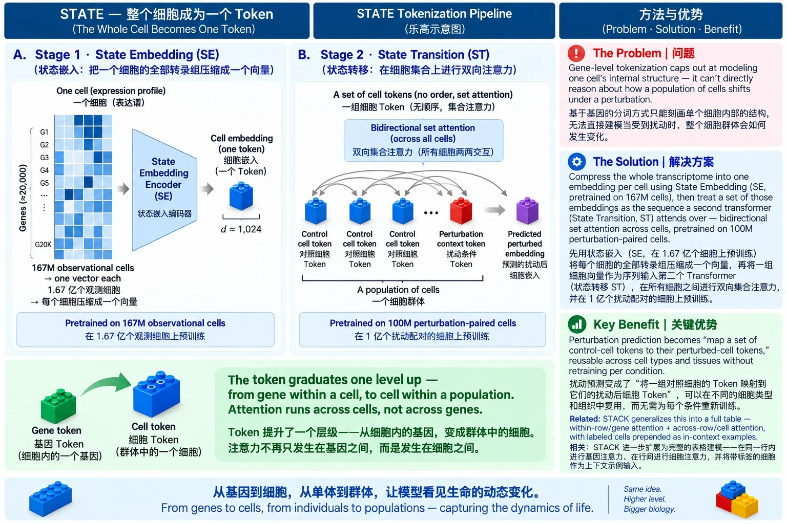
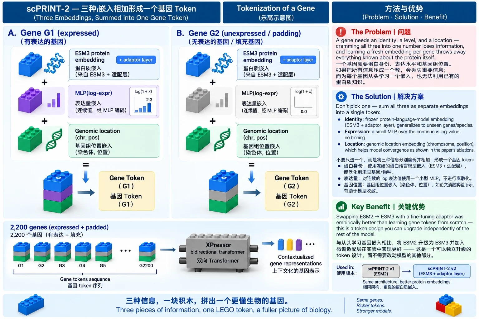
Three of the strategies above don't reduce to a single hand-drawn LEGO panel — they combine multiple embeddings per token (scPRINT-2) or move the token itself up a level, from gene to whole cell (STATE, STACK). Full walkthroughs below.
Key Papers Implementing These Strategies
Geneformer: Transfer Learning Enables Predictions in Network Biology
Tokenization Strategy
Each gene's count is divided by its corpus-wide non-zero median (down-weighting ubiquitous housekeeping genes), then genes are ranked high→low and truncated to the top 2,048 — magnitude lives entirely in token position, not in a value token.
Scale: 29.9M cells | Context: 2,048 | Params: 10.3M (original, 6-layer/256-dim; later checkpoints scale to 316M)
iSEEEK: Integration via Gene Rankings
Tokenization Strategy
Top 126 expressing genes per cell, ranked by expression level (128 total tokens = 1 [CLS] + 126 genes + 1 [SEP] — a full BERT-base-style 128-token context, not "all genes"). Uses [CLS] and [SEP] tokens with MLM objective. Vocabulary: 20,706 protein-coding genes.
Scale: 11.9M cells | Context: 128 tokens | Params: ~10M
scGPT: Multi-task Foundation Model
Tokenization Strategy
Gene tokens paired with binned expression values (51 bins). Special condition tokens for perturbation modeling. Context limited to ~1,200 most variable genes.
Scale: 33M cells | Context: 1,200 | Params: ~100M
scBERT: Large-Scale Pretrained Deep Language Model for Cell Type Annotation
Tokenization Strategy
Gene embeddings from gene2vec (fixed gene identity, not learned jointly); continuous expression values discretized into bins and embedded via term-frequency-style binning. Full-length gene input handled by a Performer (linear-attention) backbone instead of truncating to a subset.
Scale: ~1.1M cells (PanglaoDB) | Context: ~16,906 genes (full) | Architecture: 200-dim embedding, 6 Performer layers, 10 heads
Nicheformer: Spatial-Aware Foundation Model
Tokenization Strategy
Rank-based with technology-specific mean normalization. Contextual tokens: <ORGANISM>, <ASSAY>, <MODALITY>. Cross-species gene mapping via orthologs.
Scale: 110M cells | Context: 1,500 | Params: 49.3M
ChromFound: scATAC-seq Foundation Model
Tokenization Strategy
Chromosome embedding + sinusoidal positional encoding of genomic coordinates (start/end). Linear accessibility embedding. Vocabulary-free approach for dynamic OCR landscapes.
Scale: 1.97M cells | Context: 440K OCRs | Params: ~450K (confirmed against the paper's own ablation table — a genuinely compact 4-layer, 128-dim hybrid, not a typo)
DNABERT: Pre-trained Bidirectional Encoder Representations for DNA-Language in Genome
Tokenization Strategy
Overlapping sliding-window k-mers (3- to 6-mer variants tested, 4^k possible tokens), masking contiguous k-mers rather than single tokens during pretraining to prevent trivial inference from immediately adjacent, overlapping windows.
Scale: Human reference genome | Context: 512 tokens | Params: ~86-90M (12-layer BERT-base, varies by k)
DNABERT-2: Efficient Foundation Model and Benchmark for Multi-Species Genome
Tokenization Strategy
Byte-Pair Encoding merges the most frequent co-occurring subsequences into variable-length tokens (rather than fixed-width overlapping k-mer windows), so each base is covered exactly once — no k-mer overlap redundancy — while common motifs still collapse into single tokens.
Scale: Genomes from 135 species | Context: ALiBi — no fixed ceiling | Params: 117M
Evo 2: Genome Modeling and Design Across All Domains of Life
Tokenization Strategy
Every base (A/T/G/C) is its own token — no k-mer merging, no BPE vocabulary to learn or run out of. The StripedHyena 2 operator maintains a fixed-size running state instead of attending back over the full context, which is what makes single-base-per-token viable at 1Mb+ length.
Scale: 9.3T nucleotides, 128,000+ species | Context: up to 1M tokens | Params: 7B & 40B
ESM3: Multimodal Protein Language Model
Tokenization Strategy
Separate token tracks for sequence (amino acids), structure (discrete autoencoder), and function (keywords from InterPro/GO). All modalities fused in shared latent space with masked language modeling.
Scale: 2.78B proteins | Context: Sequence + 3D Structure | Params: 1.4B-98B
C2S-Scale: LLM-Scale Single-Cell Foundation
Tokenization Strategy
Cell2Sentence: expression encoded via token repetition (high expr = more repeats). GRPO refinement for biological task optimization. 8,192 token context.
Scale: 5.7M cells | Context: 8,192 | Params: 157M-27B
ProGen2: Protein Language Model Scaling
Tokenization Strategy
Standard amino acid tokenization with rotary positional encodings. Causal language modeling with next-token prediction. Context: 1,024-2,048 tokens.
Scale: UniRef90+BFD | Context: 2,048 AAs | Params: 151M-6.4B
VariantFormer: Personalized Gene Expression from Diploid Genomes
Tokenization Strategy
IUPAC ambiguity codes for heterozygous sites (R=A/G, Y=C/T, etc.) embedded into reference genome. BPE tokenizer with a deliberately small 500-token vocabulary trained on cCREs (near-character-level — minimal merging — versus the 30K–50K vocabularies typical of NLP BPE, since regulatory DNA doesn't have "words" that benefit from heavy merging). Hierarchical cross-attention between CRE (±1Mb) and gene body windows.
Scale: 2,330 donors, 50K genes | Context: >2Mb | Params: 1.2B
SATURN: Universal Cross-Species Embeddings
Tokenization Strategy
Genes clustered into ~2000 macrogenes via k-means on ESM2 protein embeddings (5120-dim). Gene-to-macrogene weights learned from protein similarity. Enables 350M-year divergent species integration.
Scale: 335K cells (3 species) | Context: ~2,000 macrogenes | Params: ~10M
State: A Scalable Virtual Cell Model Predicting Cellular Responses Across Diverse Contexts
Tokenization Strategy
Cell-as-token: each cell's full transcriptome (gene identities + expression values) is compressed into one embedding vector by SE — the gene-level tokens are upstream inputs to that encoder, not the model's sequence elements. ST then applies set attention across a batch of such cell vectors, treating each cell embedding as a "token" in the context of the cell population. Granularity is one level up from every gene-level strategy on this page. See the full diagram ↓
Scale: 167M observational + 100M perturbation cells | Context: Set-based (variable cell count) | Params: not disclosed
STACK: In-Context Learning of Single-Cell Biology
Tokenization Strategy
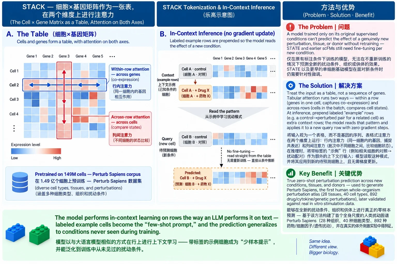
Tabular cell-as-token: the input is a cell × gene matrix, not a sequence of gene tokens. Within-cell attention (along gene columns) captures co-expression; across-cell attention (along the row dimension) compares cell states. At inference, labeled context cells are appended as additional rows — the model treats them as "few-shot examples" read directly from the table, no gradient required. Pretrained on 149M cells from the Perturb Sapiens atlas. See the full diagram ↓
Scale: 149M cells (Perturb Sapiens atlas) | Context: Tabular (variable cell count × gene count) | Params: not disclosed
tGPT: Generative Pretraining from Large-Scale Transcriptomes
Tokenization Strategy
Genes within a cell are sorted into a list by expression level, the same core move as Geneformer — no explicit expression-value token, magnitude lives in rank position. The model is then trained autoregressively (predict the next gene in the ranked list), closer to GPT-style pretraining than scBERT/Geneformer's BERT-style masking.
Scale: 22.3M cells | Context: not disclosed in this literature set | Params: not disclosed
CellPLM: Pre-training of Cell Language Model Beyond Single Cells
Tokenization Strategy
Inverts the usual gene-token paradigm — "cells as tokens, tissues as sentences": each cell (itself encoded from its gene expression) becomes one token in a sequence of cells drawn from the same tissue or spatial neighborhood, letting the transformer attend across cells the way a language model attends across words. A learned Gaussian-mixture prior regularizes the cell-token embedding space to offset scRNA-seq's data scarcity relative to text corpora.
Scale: not fully disclosed in this literature set | Context: gene tokens + cell-level batch structure | Params: not disclosed
GeneCompass: Knowledge-Informed Cross-Species Foundation Model
Tokenization Strategy
Rank-based gene tokenization in the Geneformer lineage, extended with parallel "prior-knowledge encodings" per gene — promoter-sequence, gene-family/ortholog, co-expression, and TF-target embeddings — summed alongside the expression-rank token, plus species tokens so a single shared vocabulary spans human and mouse genes via orthology mapping.
Scale: 101.8M cells (human + mouse) | Context: rank-based, Geneformer-style | Params: not disclosed
scFoundation: Large-Scale Foundation Model on Single-Cell Transcriptomics
Tokenization Strategy
Each gene's continuous, unbinned expression is embedded directly (not ranked or binned), and two extra tokens — the cell's total read count and a target read count — are added alongside the gene tokens, letting the model be told at inference time what sequencing depth to "imagine" reading at. Trained with a mixed downsampling-and-masking objective rather than plain MLM; denoising happens only at the cell-embedding level, a design later contrasted against scPRINT's per-gene denoising.
Scale: 50M cells | Context: genome-wide (~19,264 genes) | Params: ~100M (xTrimoGene encoder-decoder)
UCE: Universal Cell Embedding
Tokenization Strategy
Each cell is a weighted, with-replacement sample of 1,024 of its expressed genes — higher-expression genes are sampled more often, so expression lives in sampling frequency rather than a value token. Each gene token is the ESM2 (15B-parameter protein language model) embedding of its encoded protein, not a learned lookup — genes and species absent from training still get a meaningful token via protein-sequence homology. Gene tokens are grouped by chromosome, ordered by genomic position, and delimited by chromosome-specific start/end tokens, with a prepended CLS token whose final-layer output becomes the cell embedding.
Scale: 36M cells (IMA), 300+ datasets, cross-species | Context: 1,024 sampled gene tokens | Params: 650M (33 layers, built on frozen ESM2-15B gene tokens)
scPRINT: Pre-training on 50 Million Cells Allows Robust Gene Network Predictions
Tokenization Strategy
Each gene token is the sum of three embeddings: (1) an ESM2 protein embedding of the gene's identity — following UCE, this lets the model generalize to unseen genes and species — (2) an MLP encoding of the gene's continuous log-normalized expression (not binned or ranked, unlike scGPT/Geneformer), and (3) a genomic-location embedding. Pretrained on 2,200 randomly selected expressed genes per cell, padded with unexpressed genes when a cell has fewer — the padding lets a zero-inflated negative-binomial decoder learn to tell true biological zeros from sequencing dropout.
Scale: 50M cells (cellxgene) | Context: 2,200 genes | Params: multiple scales released
scPRINT-2: Towards the Next Generation of Cell Foundation Models and Benchmarks
Tokenization Strategy
Keeps scPRINT-1's three-way summed gene token (identity + expression + genomic location) but upgrades the identity embedding from ESM2 to ESM3, adding a fine-tuning adaptor layer after mean-pooling the protein embedding — the paper reports this beats learning gene tokens from scratch. Adds variable-context-length training and KNN-averaged "meta-cell" augmentation, plus a cell-level XPressor sub-architecture that makes the model directly generative for expression imputation and counterfactual reasoning. See the full diagram ↓
Scale: 350M cells, 16 organisms | Context: variable-length (data-augmented) | Params: not disclosed
2025–2026 developments:
· Evo 2 (2025) — single-nucleotide + StripedHyena 2 (SSM), 128,000+ species, 9.3T nucleotides, up to 1M-token context, zero k-mer OOV.
· DNABERT-2 (ICLR 2024) — BPE replaces fixed k-mer windows, eliminating overlapping-window redundancy and the fixed input-length ceiling (via ALiBi).
· Cell-level tokenization paradigm (STACK + STATE, see the Side-by-Side comparison below) — the token graduates from "gene within a cell" to "cell within a set," attending across whole cell populations rather than genes within one cell.
· VariantFormer (2025) — the first foundation model to predict tissue-specific gene expression directly from personalized diploid genomes.
· UCE (Nature 2026) — genes tokenized as ESM2 protein embeddings instead of learned IDs, giving zero-shot cross-species cell embeddings without fine-tuning.
· scPRINT / scPRINT-2 (2025–2026) — summed identity+expression+location gene tokens (ESM2 → ESM3), scaling the pretraining corpus from 50M to 350M cells across 16 organisms via an additive, one-feature-at-a-time benchmark.
Comparisons & Trade-offs
Every granularity level buys something and pays for something:
1×1 小颗粒 · Smaller units char / byte / base
✓ Zero OOV — every sequence is coverable; compositional generalization
✗ Very long sequences; almost no meaning per token; attention gets expensive
2×4 标准砖 · Middle units subword / codon / k-mer
✓ The working balance: coverage, real semantics, manageable vocabulary
✗ You must tune the knobs — merge count, k, overlapping redundancy
大板与定制件 · Larger units word / gene / macrogene
✓ Short sequences; every token carries real meaning
✗ OOV and batch-dependence; rare or novel units silently vanish
底板格点与塔高 · Value-free units rank / coordinate
✓ Batch-proof and vocabulary-free; robust across datasets
✗ Absolute magnitude is gone — 50 vs 5 becomes just 1st vs 2nd
连接件与底板 · Special tokens [CLS] / [SEP] / [MASK]
Content tokens carry meaning; special tokens carry the structure that makes meaning readable — invisible in the castle photo, but nothing snaps together without them:
[CLS] = 说明书封面的总览图 — the single overview picture that summarizes the whole build (classification & sequence embedding)
[SEP] = 房间隔断砖 — divider bricks that split one build into readable rooms (segment boundaries)
[MASK] = 被遮住的那一格 — a covered slot the model must guess from the surrounding bricks (where the learning signal comes from)
The table below is the same trade-off, one strategy at a time:
Tokenization Strategy Comparison
| Strategy | Data Type | Key Advantage | Limitation | Representative Model |
|---|---|---|---|---|
| Gene Rank-Based | scRNA-seq | Batch-insensitive, captures relative expression patterns | Loses absolute expression magnitude | iSEEEK, Geneformer |
| Expression Binning | scRNA-seq | Preserves expression magnitude, compatible with NLP architectures | Information loss from discretization | scGPT, scBERT |
| Genome-Coordinate | scATAC-seq | Vocabulary-free, handles novel regions | Requires reference genome alignment | ChromFound |
| K-mer Tokenization | DNA sequences | Captures local sequence patterns | Large vocabulary (4^k tokens) | Nucleotide Transformer |
| BPE + IUPAC | Diploid DNA + Variants | Native heterozygous encoding; personalized genome modeling | Requires phased VCF; expanded alphabet | VariantFormer |
| Amino Acid + Multimodal | Protein sequences + structure + function | Simple sequence tokens; multimodal enables structure/function reasoning | Ignores codon usage effects | ESM3, ProGen2 |
| Cell2Sentence | scRNA-seq | Compatible with standard LLMs, enables NL queries | Long sequences from repetition encoding | C2S-Scale |
| Macrogene | scRNA-seq (cross-species) | Enables cross-species integration without homologs via protein embeddings | Requires reference proteomes; loses gene-level resolution | SATURN |
| Single-Nucleotide + SSM | DNA (genomic, long-context) | Zero OOV (4-symbol vocabulary); no k-mer overlap redundancy; linear-time scan to 1M+ bp | Requires a state-space architecture (Hyena/Mamba), not a plain Transformer | Evo 2, HyenaDNA |
| Cell-as-Token (Set / Tabular) | scRNA-seq | Attends across whole cell populations; enables in-context perturbation prediction without fine-tuning | Token is an entire cell — requires a cell-level encoder upstream of the set/tabular operator | State, STACK |
Context Length vs Model Scale Trade-offs
Different tokenization strategies and architectures dictate the maximum sequence length (context window) a model can handle, which impacts the biological scope it can capture.
| Model | Tokenization Strategy | Context Length | Parameters |
|---|---|---|---|
| iSEEEK | Rank-Based (Top-K) | 128 tokens | ~10M |
| scGPT | Binning (High Variance Genes) | ~1,200 genes | ~100M |
| Nicheformer | Rank-Based (Top-K) | 1,500 tokens | 49.3M |
| AIDO.Cell | Auto-Discretization (Full Transcriptome) | 19,264 (full) | 650M |
| ChromFound | Genome-Coordinate (OCRs) | 440K OCRs (via Mamba) | 450K |
| ESM3 | Amino Acid + Structure + Function | Full protein (multimodal) | 98B |
| VariantFormer | BPE + IUPAC (Diploid) | >2 Mb (CRE ±1Mb + gene body) | 1.2B |
| C2S-Scale | Cell2Sentence (Repetition) | 8,192 tokens | 27B |
| SATURN | Macrogene (ESM2-based) | ~2,000 macrogenes | ~10M |
| Evo 2 | Single-Nucleotide (StripedHyena 2 SSM) | up to 1M tokens | 7B / 40B |
| State | Cell-as-Token (Set Transformer) | Set-based (variable — whole cell population) | not disclosed |
| STACK | Cell-as-Token (Tabular ICL) | Tabular (variable cells × ~20K genes) | not disclosed |
Choosing the Right Tokenization Strategy
| Use Case | Recommended Strategy | Why |
|---|---|---|
| Large-scale integration (>1M cells) across many labs | Gene Rank-Based | Naturally batch-insensitive; focuses on robust relative signals. |
| Perturbation modeling (predicting gene knockout effects) | Expression Binning | Preserves the absolute expression magnitude needed to model dosage changes. |
| Chromatin accessibility analysis (scATAC-seq) | Genome-Coordinate Tokenization | Handles dynamic open chromatin regions varying across cell types without a fixed vocabulary. |
| Protein fitness or structure prediction | Amino Acid Tokenization | Standard approach that effectively captures evolutionary constraints in protein sequences. |
| Personalized gene expression prediction from WGS | BPE + IUPAC | Encodes heterozygous variants natively; enables variant effect prediction from individual genomes. |
| Interacting with cell data using natural language | Cell2Sentence | Converts biological data into a format understood by standard Large Language Models. |
| Whole-genome or chromosome-scale long-sequence analysis | Single-Nucleotide + SSM | K-mer vocabularies explode at 1M+ context; a state-space model's linear scaling is the only tractable path at that length. |
| Cross-species comparative genomics without 1:1 orthologs | Macrogene | Clustering by protein-embedding similarity bridges species separated by hundreds of millions of years of divergence. |
| Perturbation prediction across new conditions / tissues without fine-tuning | Cell-as-Token (STACK) | Tabular in-context learning reads labeled example cells at inference — no gradient update needed for new perturbations or donors. |
⚖️ Side-by-Side: Encoding Expression — Rank Ordering vs Value Binning
Geneformer and scGPT both turn a single cell's expression vector into a token sequence a transformer can read, but they diverge on the fundamental question: should a gene's expression level be encoded implicitly by its rank among the other genes (Geneformer), or explicitly as a discrete value token paired with the gene (scGPT)?
The same starting point — one cell's gene-by-count vector — becomes two very different token streams depending on how expression magnitude is represented:
The split traces back to one root decision — rank ordering vs value binning. Geneformer discards absolute magnitude (50 vs 5 collapses to just 1st vs 2nd), which makes it naturally depth- and batch-robust but blind to dosage; scGPT keeps magnitude as an explicit token, which is exactly what perturbation and dosage modeling need but leaves it sensitive to normalization and batch. Vocabulary size, sequence length, and out-of-vocabulary behavior all follow from that one choice.
Up a Level: Cells as Tokens — STACK vs STATE
The two models above tokenize genes within a cell. STACK and STATE (both from the Arc Institute) move up a granularity — the token is the whole cell, and attention runs over a set or table of cells. They diverge on how a set of cells becomes a perturbation prediction: STACK learns in context from unlabeled example cells at inference, while STATE trains an explicit embedding-plus-transition pipeline.
The same set of cells becomes a perturbation prediction two different ways — by learning in context at inference, or by a separately trained transition operator:
The root decision here is in-context learning from example cells vs a separately trained embedding-and-transition pipeline. Both treat the cell (not the gene) as the token and attend across a set of cells — a step up in granularity from the gene-level tokens above. STACK trades a training step for flexible, fine-tuning-free generalization to new conditions; STATE's dedicated transition model gives an explicit control→perturbed operator built specifically for perturbation-effect prediction.
🛠️ Hands-On Practice
The steps below walk through tokenizing a single-cell dataset for a transformer foundation model — from an AnnData count matrix to two model-ready token streams: a rank-ordered sequence (Geneformer-style) and a (gene, value-bin) sequence (scGPT-style). The core logic is shown from scratch in NumPy so the mechanics are transparent, then mapped to the real library call.
Environment & packages
Install a minimal tokenization stack. scanpy/anndata hold the matrix; the model-specific tokenizers (Geneformer's TranscriptomeTokenizer, scGPT's GeneVocab) emit the final token IDs and handle the gene vocabulary, special tokens, and truncation.
# conda / mamba recommended
conda create -n tok python=3.10 -y
conda activate tok

pip install scanpy anndata numpy datasets
# model-specific tokenizers:
pip install geneformer          # rank-value encoding (expects Ensembl IDs)
# pip install scgpt             # value binning (GeneVocab tokenizer)
Hardware. Tokenization is CPU-bound and cheap — a laptop handles 100k+ cells. A GPU is only needed for the downstream model forward pass, not for building the token streams.
Data structures & formats
AnnData— input:adata.X(raw counts),adata.var["ensembl_id"](Geneformer keys on Ensembl IDs, not symbols),adata.obs["n_counts"](total counts per cell)- Token dictionary — a fixed
gene → integer IDvocabulary; genes absent from it are out-of-vocabulary and silently dropped - Rank-encoded sequence — an ordered list of gene token IDs per cell (no value tokens), truncated to the model context length (2,048 for Geneformer)
- Value-binned sequence — aligned arrays of gene token IDs and discrete value-bin IDs (e.g. 51 bins) per cell
- Special tokens —
<cls>(cell-level embedding),<pad>(padding to a fixed length),<mask>(masked-token pretraining objective) - Output — Geneformer emits a HuggingFace
.dataset(Arrow) of token IDs; scGPT works from tensors of(gene_ids, values)
Minimal code walkthrough
Encode a toy count matrix with both strategies to expose the mechanics, then map to the real Geneformer tokenizer.
import numpy as np

# Toy: 3 cells x 6 genes (raw UMI counts). In practice: adata = sc.read_h5ad(...)
genes  = np.array(["CD3D", "MS4A1", "GAPDH", "NKG7", "LYZ", "ACTB"])
counts = np.array([[12,  0, 40, 3,  0, 30],
                   [ 0, 25, 35, 1, 18, 22],
                   [ 5,  0, 50, 9,  2, 28]], dtype=float)

# ---------- Strategy A: rank-value encoding (Geneformer-style) ----------
# 1. Normalize each gene by its NON-ZERO median across the corpus. This
#    down-weights housekeeping genes that are uniformly high (GAPDH, ACTB).
nz          = np.where(counts > 0, counts, np.nan)
gene_median = np.nanmedian(nz, axis=0)
norm        = counts / gene_median

# 2. Per cell, rank genes by normalized expression high -> low; drop zeros.
def rank_encode(cell):
    idx = np.where(cell > 0)[0]
    return genes[idx[np.argsort(-cell[idx])]].tolist()

for i in range(counts.shape[0]):
    print(f"cell {i} rank tokens:", rank_encode(norm[i]))
# -> ordered gene tokens only; magnitude lives in POSITION, no value token.

# ---------- Strategy B: value binning (scGPT-style) ----------
N_BINS = 5   # scGPT uses ~51 in practice
def value_bin(cell):
    idx   = np.where(cell > 0)[0]
    vals  = np.log1p(cell[idx])
    ranks = vals.argsort().argsort()                 # per-cell quantile rank
    bins  = np.floor(ranks / len(idx) * N_BINS).astype(int)
    bins  = np.clip(bins, 0, N_BINS - 1)              # guard the top-rank edge case
    return list(zip(genes[idx].tolist(), bins.tolist()))

for i in range(counts.shape[0]):
    print(f"cell {i} (gene, bin):", value_bin(counts[i]))
# -> aligned (gene token, value-bin token) pairs; magnitude is explicit.
In production you would not hand-roll this — the model ships a tokenizer that also handles the gene vocabulary, special tokens, and truncation:
# tested against geneformer>=1.0 — the TranscriptomeTokenizer constructor
# signature has changed across major versions; pin your version and check
# the CHANGELOG before upgrading an existing tokenization pipeline.
from geneformer import TranscriptomeTokenizer

# adata must carry raw counts, adata.var["ensembl_id"], adata.obs["n_counts"].
tk = TranscriptomeTokenizer({"cell_type": "cell_type"}, nproc=4)
tk.tokenize_data(
    "data_dir/",        # folder of .h5ad / .loom files
    "output_dir/",
    "tokenized",        # output prefix
    file_format="h5ad",
)
# -> output_dir/tokenized.dataset : rank-ordered token IDs per cell,
#    median-normalized internally and truncated to 2,048 genes.
Strategy C: single-nucleotide tokenization (Evo/HyenaDNA-style). For DNA rather than expression data, the same "hand-roll it first" approach looks like this — no gene vocabulary, no binning, just one token per base:
# Vocab = 5 (4 bases + N for ambiguous/unknown); no merge operations at all.
nuc_vocab = {"A": 0, "T": 1, "G": 2, "C": 3, "N": 4}

def nucleotide_tokenize(seq: str) -> list[int]:
    return [nuc_vocab.get(c.upper(), 4) for c in seq]

seq = "ATGCATGCN..."   # in practice: a 1Mb+ window read from a reference/FASTA
tokens = nucleotide_tokenize(seq)
# -> every character becomes a token; zero OOV by construction, but the
#    context length equals len(seq) exactly — at genome scale this is only
#    tractable with a linear-time backend (Hyena/Mamba), not full attention.
Common pitfalls & tips
- Gene ID system mismatch. Geneformer's vocabulary is keyed on Ensembl IDs, not gene symbols — map symbols → Ensembl before tokenizing, or most genes become OOV and vanish.
- Wrong normalization state. Geneformer expects raw counts and median-normalizes internally; scGPT expects normalized/log1p input. Double-normalizing (feeding already-log-normed data to Geneformer) corrupts the ranking.
- Check vocabulary coverage. Any gene not in the token dictionary is dropped silently; a low-overlap panel (targeted or non-human data) can lose most of its signal before the model sees a single token. Log the fraction of counts retained.
- Sequence-length truncation drops the tail. Rank encoding keeps only the top ~2,048 genes; lowly expressed but biologically important genes fall off the end, and sparse cells yield short, padding-heavy sequences.
- Value bins are per-cell and relative. "Bin 50" in one cell is not the same absolute expression as "bin 50" in another — binning is computed within each cell, so depth and batch effects shift the mapping; don't compare raw bin IDs across cells.
- Don't forget special tokens. The
<cls>position carries the cell-level embedding and<pad>must be masked in attention; omitting or mis-placing them silently degrades every downstream readout.